Data Structures and Algorithms Graph Algorithms II Gal

Data Structures and Algorithms Graph Algorithms II Gal A. Kaminka Computer Science Department 1

Representing a relation l l l Given a set S Given a mathematical relation R on S x S We can represent R as a directed graph as follows l l l Gr = < V, E > V=S E = { <e 1, e 2> | e 1, e 2 in S, (e 1, e 2) in R } 2

Partial and total orders l l R can represent a partial order, or total order Partial order: l l <a, b>, <c, b>, and unknown <a, c> nor <c, a> In graph: <a, b>, <c, b> and not <a, c>, <c, a> Sometimes called precedence relationship Total order: l <a, b> <c, b> implies either <a, c> or <c, a> exists 3

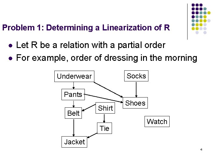
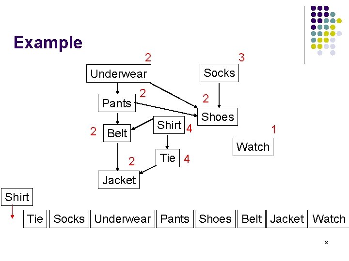
Problem 1: Determining a Linearization of R l l Let R be a relation with a partial order For example, order of dressing in the morning Socks Underwear Pants Belt Shirt Tie Shoes Watch Jacket 4

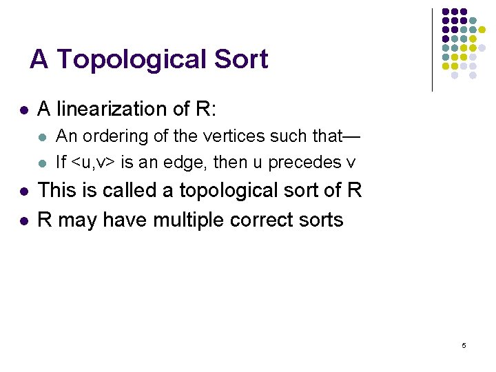
A Topological Sort l A linearization of R: l l An ordering of the vertices such that— If <u, v> is an edge, then u precedes v This is called a topological sort of R R may have multiple correct sorts 5

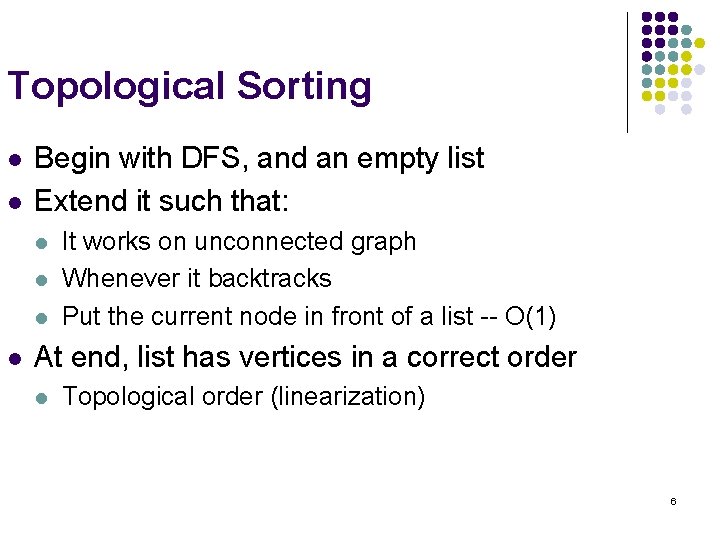
Topological Sorting l l Begin with DFS, and an empty list Extend it such that: l l It works on unconnected graph Whenever it backtracks Put the current node in front of a list -- O(1) At end, list has vertices in a correct order l Topological order (linearization) 6

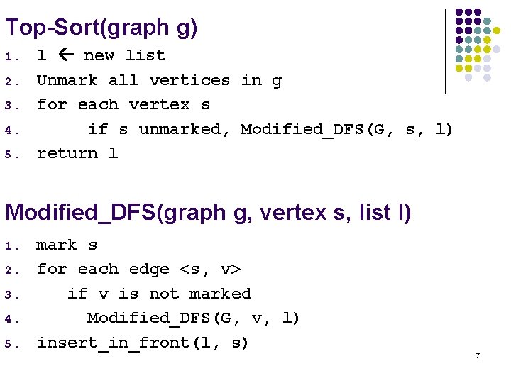
Top-Sort(graph g) 1. 2. 3. 4. 5. l new list Unmark all vertices in g for each vertex s if s unmarked, Modified_DFS(G, s, l) return l Modified_DFS(graph g, vertex s, list l) 1. 2. 3. 4. 5. mark s for each edge <s, v> if v is not marked Modified_DFS(G, v, l) insert_in_front(l, s) 7

Example 2 Underwear Pants 3 Socks 2 2 Shirt 4 2 Belt 2 Tie 4 Shoes 1 Watch Jacket Shirt Tie Socks Underwear Pants Shoes Belt Jacket Watch 8

Problem 2: All reachable vertices l l Suppose we are given a graph G, and a vertex v We want: What vertices reachable from v? Reachable(G, v) 1. l new list 2. Unmark all vertices in G 3. Modified_DFS(G, v, l) 4. return l 9

Problem 3: Computing transitive closure The transitive closure of G: l A graph G* is the transitive closure of G iff l For any two edges <a, b>, <b, c> there exists <a, c> l i. e. , <a, b> in G*, if path exists from a to b in G. How can we find the transitive closure of G? 10

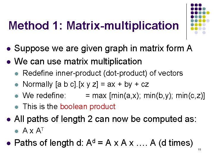
Method 1: Matrix-multiplication l l Suppose we are given graph in matrix form A We can use matrix multiplication l l l All paths of length 2 can now be computed as: l l Redefine inner-product (dot-product) of vectors Normally [a b c]. [x y z] = ax + by + cz We redefine: = max [min(a, x); min(b, y); min(c, z)] This is the boolean product A x AT Paths of length d: Ad = A x …. A (d times) 11

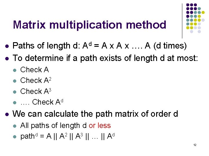
Matrix multiplication method l l Paths of length d: Ad = A x …. A (d times) To determine if a path exists of length d at most: l l l Check A 2 Check A 3 …. Check Ad We can calculate the path matrix of order d l l All paths of length d or less pathd = A || A 2 || A 3 || … || Ad 12

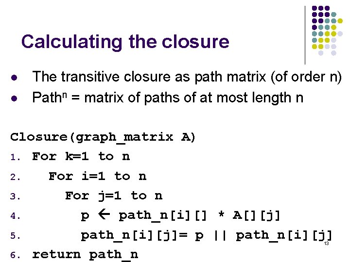
Calculating the closure l l The transitive closure as path matrix (of order n) Pathn = matrix of paths of at most length n Closure(graph_matrix A) 1. For k=1 to n 2. For i=1 to n 3. For j=1 to n 4. p path_n[i][] * A[][j] 5. path_n[i][j]= p || path_n[i][j] 6. return path_n 13

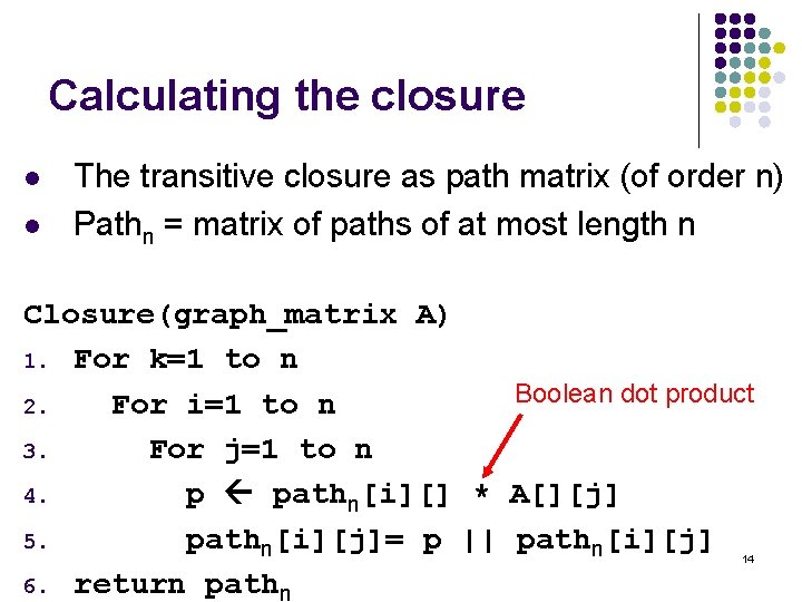
Calculating the closure l l The transitive closure as path matrix (of order n) Pathn = matrix of paths of at most length n Closure(graph_matrix A) 1. For k=1 to n Boolean dot product 2. For i=1 to n 3. For j=1 to n 4. p pathn[i][] * A[][j] 5. pathn[i][j]= p || pathn[i][j] 6. return pathn 14

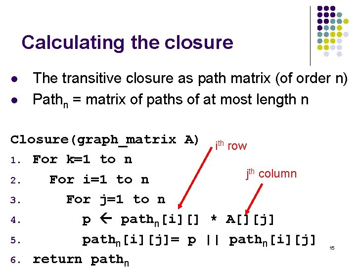
Calculating the closure l l The transitive closure as path matrix (of order n) Pathn = matrix of paths of at most length n Closure(graph_matrix A) ith row 1. For k=1 to n th column j 2. For i=1 to n 3. For j=1 to n 4. p pathn[i][] * A[][j] 5. pathn[i][j]= p || pathn[i][j] 6. return pathn 15

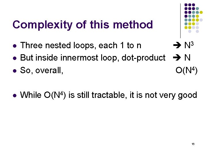
Complexity of this method l Three nested loops, each 1 to n N 3 But inside innermost loop, dot-product N So, overall, O(N 4) l While O(N 4) is still tractable, it is not very good l l 16

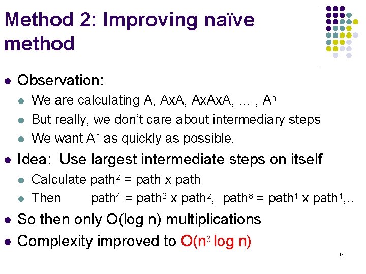
Method 2: Improving naïve method l Observation: l l Idea: Use largest intermediate steps on itself l l We are calculating A, Ax. Ax. A, … , An But really, we don’t care about intermediary steps We want An as quickly as possible. Calculate path 2 = path x path Then path 4 = path 2 x path 2, path 8 = path 4 x path 4, . . So then only O(log n) multiplications Complexity improved to O(n 3 log n) 17

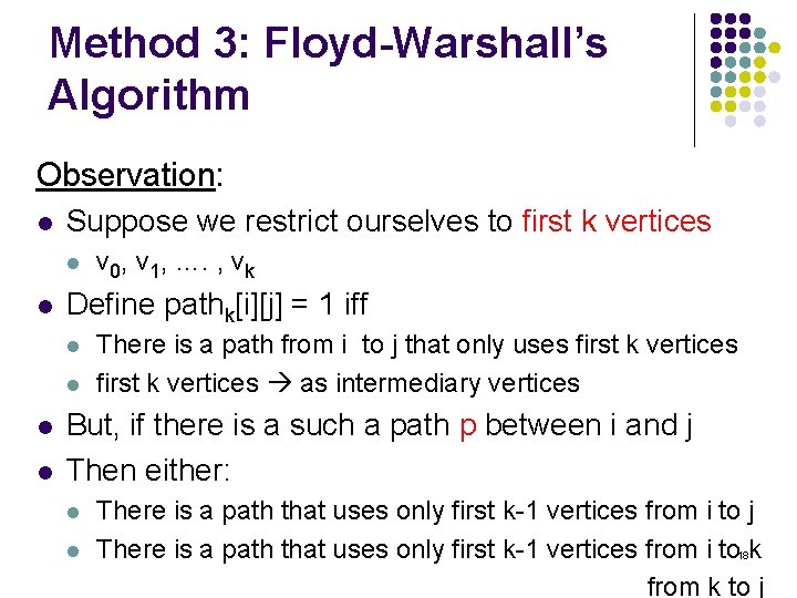
Method 3: Floyd-Warshall’s Algorithm Observation: l Suppose we restrict ourselves to first k vertices l l Define pathk[i][j] = 1 iff l l v 0, v 1, …. , vk There is a path from i to j that only uses first k vertices as intermediary vertices But, if there is a such a path p between i and j Then either: l l There is a path that uses only first k-1 vertices from i to j There is a path that uses only first k-1 vertices from i to 18 k from k to j

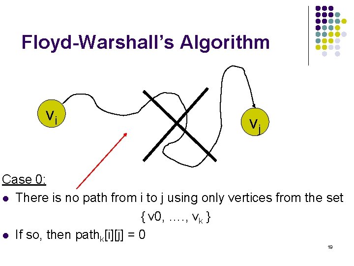
Floyd-Warshall’s Algorithm vi vj Case 0: l There is no path from i to j using only vertices from the set { v 0, …. , vk } l If so, then pathk[i][j] = 0 19

pathk[i][j] = 1 vi vj Case 1: l There is a path from i to j using only vertices from the set { v 0, …. , vk-1 } l If so, then pathk-1[i][j] = 1 20

pathk[i][j] = 1 vi vk vj Case 2: l There is a path from i to j which uses vertex vk, and vertices from the set { v 0, …. , vk-1 } l If so, then pathk-1[i][k] = 1 AND pathk-1[k][j] = 1 21

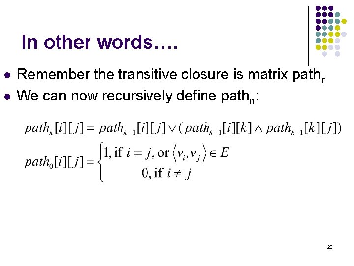
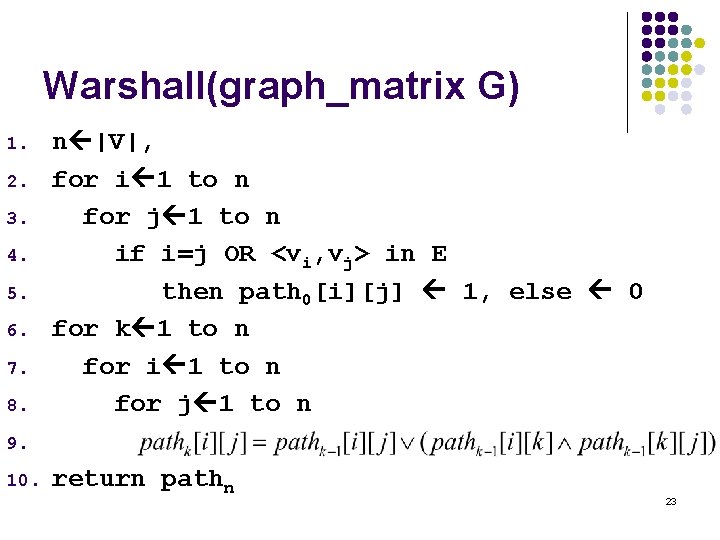
In other words…. l l Remember the transitive closure is matrix pathn We can now recursively define pathn: 22

Warshall(graph_matrix G) 1. 2. 3. 4. 5. 6. 7. 8. n |V|, for i 1 to n for j 1 to n if i=j OR <vi, vj> in E then path 0[i][j] 1, else 0 for k 1 to n for i 1 to n for j 1 to n 9. 10. return pathn 23

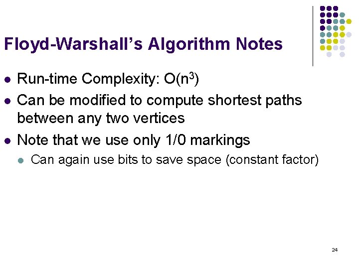
Floyd-Warshall’s Algorithm Notes l l l Run-time Complexity: O(n 3) Can be modified to compute shortest paths between any two vertices Note that we use only 1/0 markings l Can again use bits to save space (constant factor) 24