CS 235102 Data Structures Chapter 6 Graphs Chapter

CS 235102 Data Structures Chapter 6 Graphs

Chapter 6 Graphs: Outline § The Graph Abstract Data Type § Graph Representations § Elementary Graph Operations § Depth First and Breadth First Search § Spanning Tree § Minimum Cost Spanning Trees § Kruskal’s, Prim’s and Sollin’s Algorithm § Shortest Paths § Transitive Closure § Topological Sorts § Activity Networks § Critical Paths

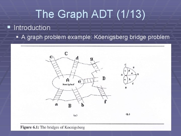
The Graph ADT (1/13) § Introduction § A graph problem example: Köenigsberg bridge problem

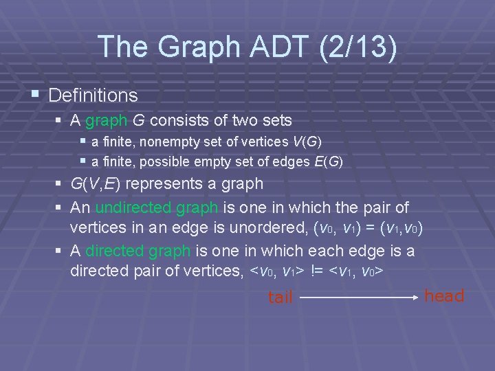
The Graph ADT (2/13) § Definitions § A graph G consists of two sets § a finite, nonempty set of vertices V(G) § a finite, possible empty set of edges E(G) § G(V, E) represents a graph § An undirected graph is one in which the pair of vertices in an edge is unordered, (v 0, v 1) = (v 1, v 0) § A directed graph is one in which each edge is a directed pair of vertices, <v 0, v 1> != <v 1, v 0> tail head

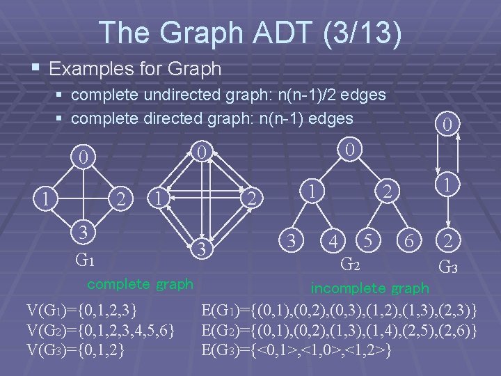
The Graph ADT (3/13) § Examples for Graph § complete undirected graph: n(n-1)/2 edges § complete directed graph: n(n-1) edges 1 0 0 0 2 1 3 G 1 complete graph V(G 1)={0, 1, 2, 3} V(G 2)={0, 1, 2, 3, 4, 5, 6} V(G 3)={0, 1, 2} 1 2 3 0 3 1 2 5 4 G 2 6 2 G 3 incomplete graph E(G 1)={(0, 1), (0, 2), (0, 3), (1, 2), (1, 3), (2, 3)} E(G 2)={(0, 1), (0, 2), (1, 3), (1, 4), (2, 5), (2, 6)} E(G 3)={<0, 1>, <1, 0>, <1, 2>}

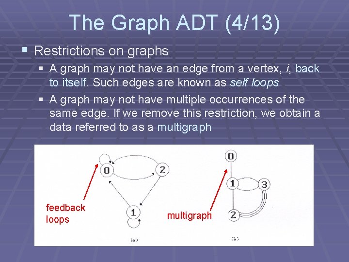
The Graph ADT (4/13) § Restrictions on graphs § A graph may not have an edge from a vertex, i, back to itself. Such edges are known as self loops § A graph may not have multiple occurrences of the same edge. If we remove this restriction, we obtain a data referred to as a multigraph feedback loops multigraph

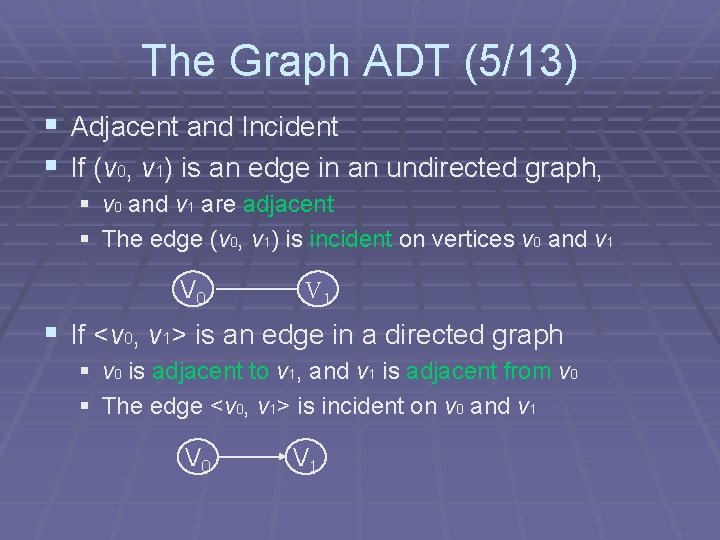
The Graph ADT (5/13) § Adjacent and Incident § If (v 0, v 1) is an edge in an undirected graph, § v 0 and v 1 are adjacent § The edge (v 0, v 1) is incident on vertices v 0 and v 1 V 0 V 1 § If <v 0, v 1> is an edge in a directed graph § v 0 is adjacent to v 1, and v 1 is adjacent from v 0 § The edge <v 0, v 1> is incident on v 0 and v 1 V 0 V 1

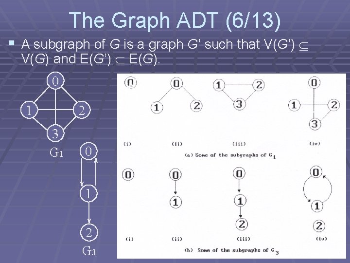
The Graph ADT (6/13) § A subgraph of G is a graph G’ such that V(G’) V(G) and E(G’) E(G). 0 1 2 3 G 1 0 1 2 G 3

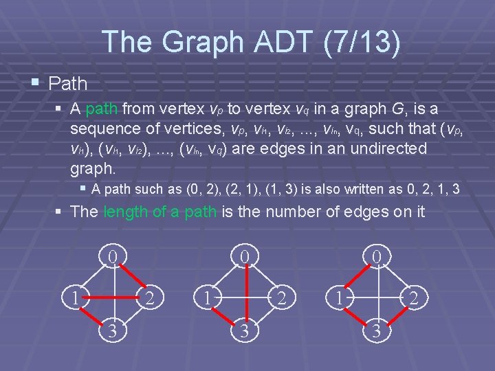
The Graph ADT (7/13) § Path § A path from vertex vp to vertex vq in a graph G, is a sequence of vertices, vp, vi 1, vi 2, . . . , vin, vq, such that (vp, vi 1), (vi 1, vi 2), . . . , (vin, vq) are edges in an undirected graph. § A path such as (0, 2), (2, 1), (1, 3) is also written as 0, 2, 1, 3 § The length of a path is the number of edges on it 0 1 0 2 3 1 2 3

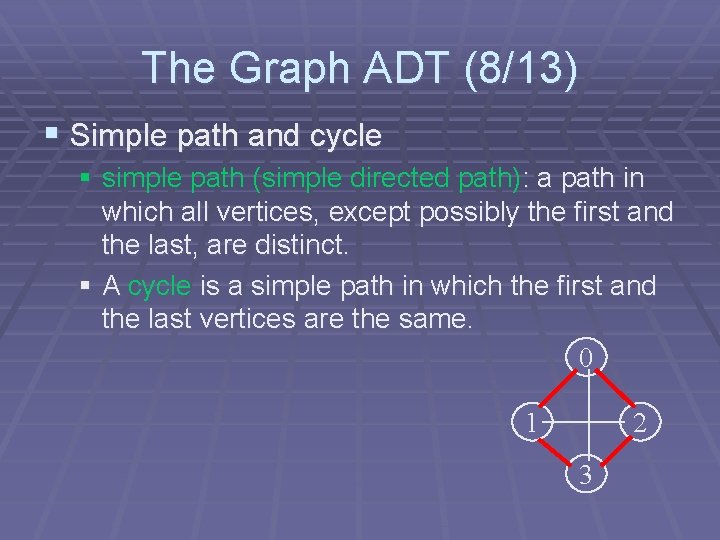
The Graph ADT (8/13) § Simple path and cycle § simple path (simple directed path): a path in which all vertices, except possibly the first and the last, are distinct. § A cycle is a simple path in which the first and the last vertices are the same. 0 1 2 3

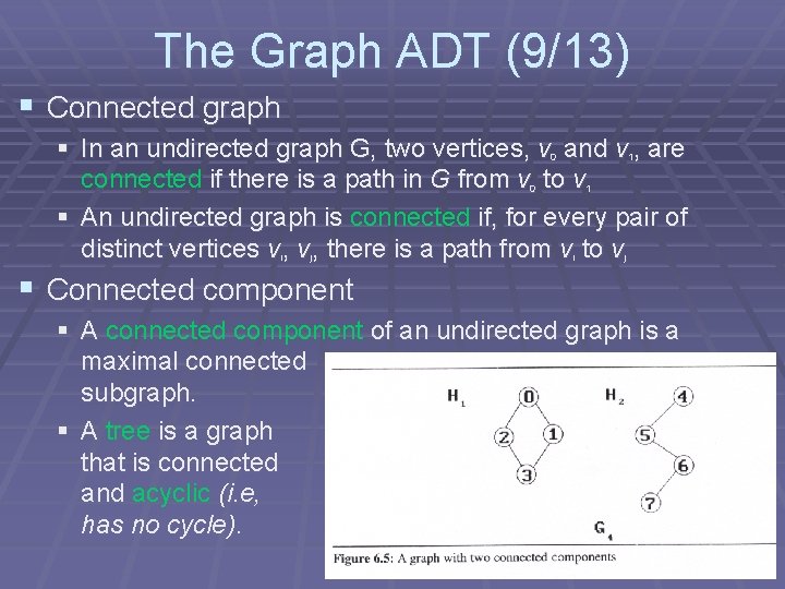
The Graph ADT (9/13) § Connected graph § In an undirected graph G, two vertices, v and v , are connected if there is a path in G from v to v § An undirected graph is connected if, for every pair of distinct vertices v , there is a path from v to v 0 1 0 i j 1 i j § Connected component § A connected component of an undirected graph is a maximal connected subgraph. § A tree is a graph that is connected and acyclic (i. e, has no cycle).

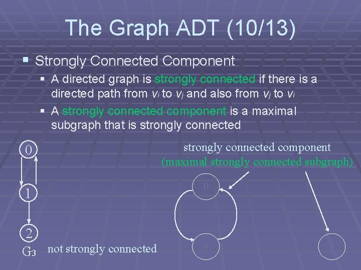
The Graph ADT (10/13) § Strongly Connected Component § A directed graph is strongly connected if there is a directed path from vi to vj and also from vj to vi § A strongly connected component is a maximal subgraph that is strongly connected 0 1 2 G 3 not strongly connected component (maximal strongly connected subgraph) 0 1 2

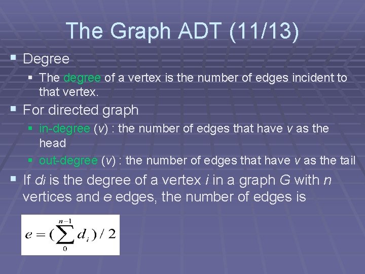
The Graph ADT (11/13) § Degree § The degree of a vertex is the number of edges incident to that vertex. § For directed graph § in-degree (v) : the number of edges that have v as the head § out-degree (v) : the number of edges that have v as the tail § If di is the degree of a vertex i in a graph G with n vertices and e edges, the number of edges is

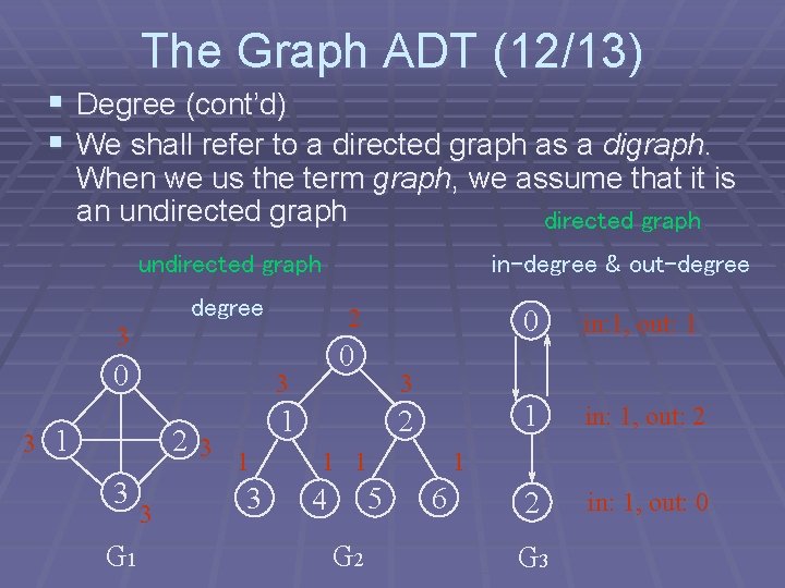
The Graph ADT (12/13) § Degree (cont’d) § We shall refer to a directed graph as a digraph. When we us the term graph, we assume that it is an undirected graph in-degree & out-degree 2 3 0 3 1 2 3 1 3 3 3 G 1 0 3 2 1 1 5 G 2 in: 1, out: 1 1 in: 1, out: 2 2 in: 1, out: 0 3 1 4 0 1 6 G 3

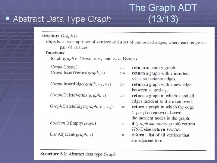
§ Abstract Data Type Graph The Graph ADT (13/13)

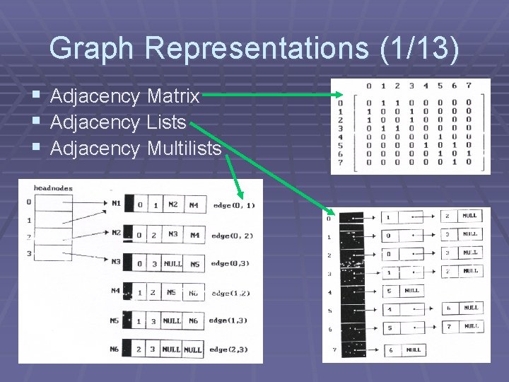
Graph Representations (1/13) § § § Adjacency Matrix Adjacency Lists Adjacency Multilists

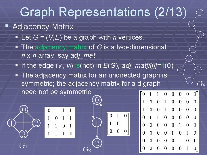
Graph Representations (2/13) 4 5 § Adjacency Matrix 6 § Let G = (V, E) be a graph with n vertices. § The adjacency matrix of G is a two-dimensional 7 n x n array, say adj_mat 0 § If the edge (vi, vj) is(not) in E(G), adj_mat[i][j]=1 ]= (0) 1 2 § The adjacency matrix for an undirected graph is 3 G 4 symmetric; the adjacency matrix for a digraph need not be symmetric 0 0 1 1 2 3 G 1 G 3 2

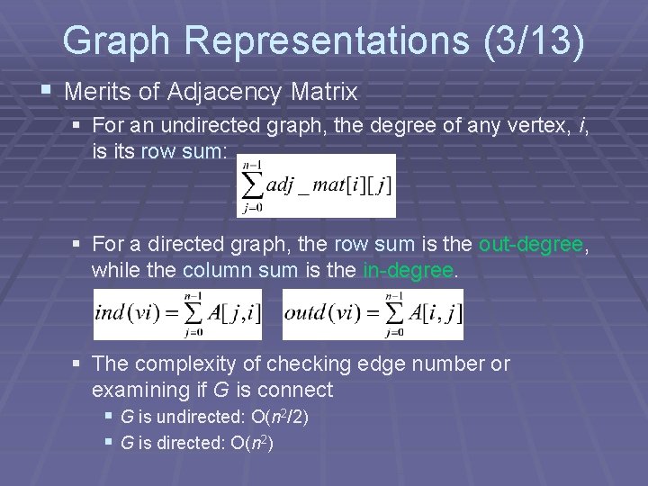
Graph Representations (3/13) § Merits of Adjacency Matrix § For an undirected graph, the degree of any vertex, i, is its row sum: § For a directed graph, the row sum is the out-degree, while the column sum is the in-degree. § The complexity of checking edge number or examining if G is connect § G is undirected: O(n 2/2) § G is directed: O(n 2)

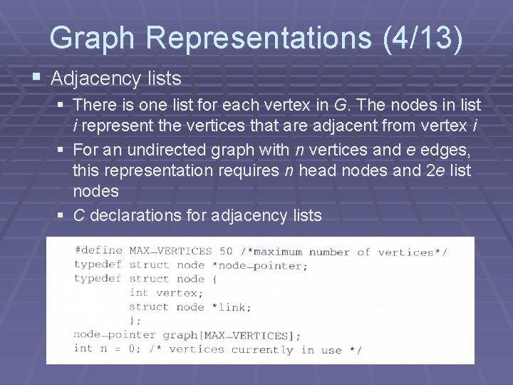
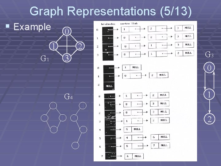
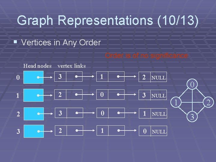
Graph Representations (4/13) § Adjacency lists § There is one list for each vertex in G. The nodes in list i represent the vertices that are adjacent from vertex i § For an undirected graph with n vertices and e edges, this representation requires n head nodes and 2 e list nodes § C declarations for adjacency lists

Graph Representations (5/13) § Example 0 1 2 3 G 1 G 3 0 1 G 4 4 0 1 2 5 2 6 3 7

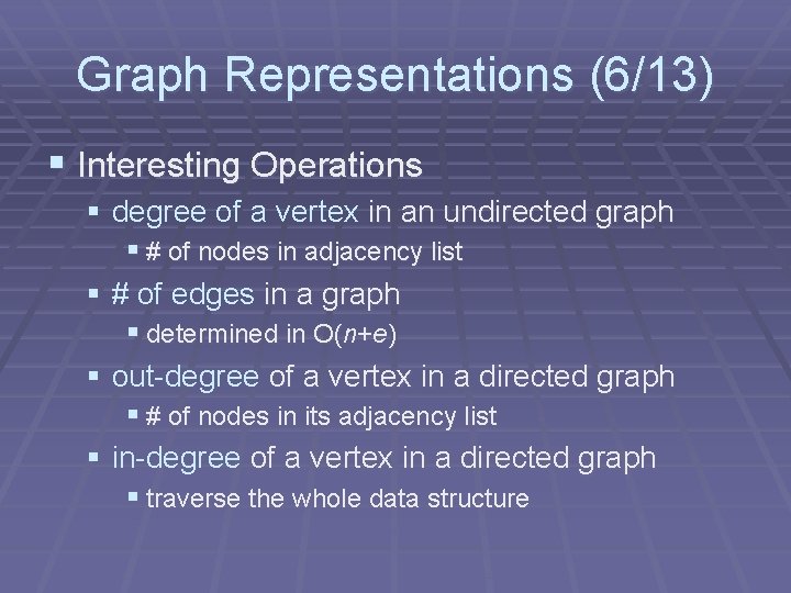
Graph Representations (6/13) § Interesting Operations § degree of a vertex in an undirected graph § # of nodes in adjacency list § # of edges in a graph § determined in O( +e) § out-degree of a vertex in a directed graph § # of nodes in its adjacency list § in-degree of a vertex in a directed graph § traverse the whole data structure

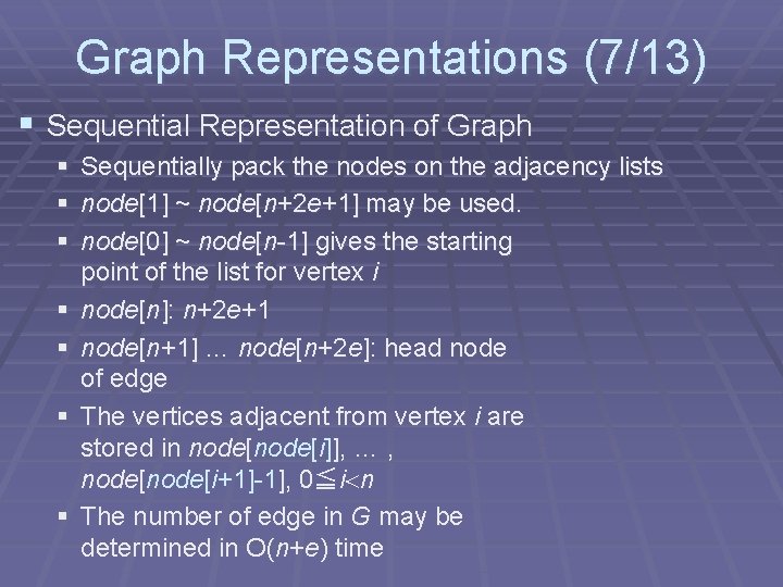
Graph Representations (7/13) § Sequential Representation of Graph § § § § Sequentially pack the nodes on the adjacency lists node[1] ~ node[n+2 e+1] may be used. node[0] ~ node[n-1] gives the starting point of the list for vertex i node[n]: n+2 e+1 node[n+1] … node[n+2 e]: head node of edge The vertices adjacent from vertex i are stored in node[i]], … , node[i+1]-1], 0≦i n The number of edge in G may be determined in O(n+e) time

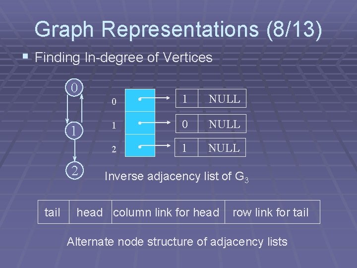
Graph Representations (8/13) § Finding In-degree of Vertices 0 1 2 tail 0 1 NULL 1 0 NULL 2 1 NULL Inverse adjacency list of G 3 head column link for head row link for tail Alternate node structure of adjacency lists

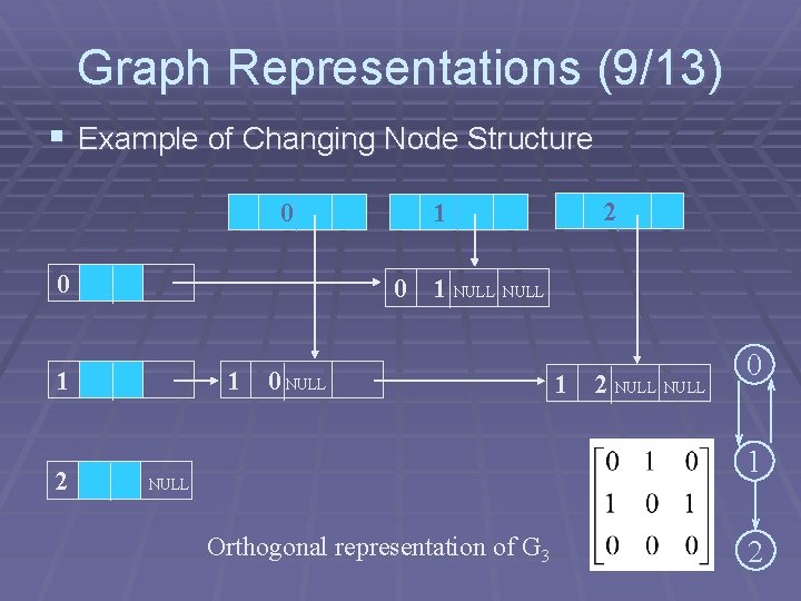
Graph Representations (9/13) § Example of Changing Node Structure 0 0 0 1 2 1 1 NULL 0 NULL 1 2 NULL 0 1 NULL Orthogonal representation of G 3 2

Graph Representations (10/13) § Vertices in Any Order is of no significance Head nodes vertex links 0 3 1 2 NULL 1 2 0 3 NULL 2 3 0 1 NULL 3 2 1 0 NULL 0 1 2 3

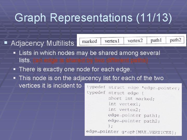
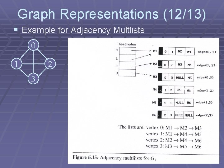
Graph Representations (11/13) § Adjacency Multilists § Lists in which nodes may be shared among several lists. (an edge is shared by two different paths) § There is exactly one node for each edge. § This node is on the adjacency list for each of the two vertices it is incident to

Graph Representations (12/13) § Example for Adjacency Multlists 0 1 2 3

Graph Representations (13/13) § Weighted edges § The edges of a graph have weights assigned to them. § These weights may represent as § the distance from one vertex to another § cost of going from one vertex to an adjacent vertex. § adjacency matrix: adj_mat[i][j] would keep the weights. § adjacency lists: add a weight field to the node structure. § A graph with weighted edges is called a network

Graph Operations (1/20) § Traversal Given G=(V, E) and vertex v, find all w V, such that w connects v § Depth First Search (DFS): preorder traversal § Breadth First Search (BFS): level order traversal § Spanning Trees § Biconnected Components

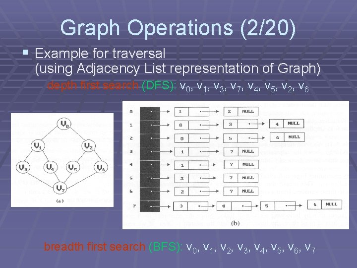
Graph Operations (2/20) § Example for traversal (using Adjacency List representation of Graph) depth first search (DFS): v 0, v 1, v 3, v 7, v 4, v 5, v 2, v 6 breadth first search (BFS): v 0, v 1, v 2, v 3, v 4, v 5, v 6, v 7

§ Depth First Search w Data structure adjacency list: O(e) adjacency matrix: O(n 2) #define FALSE 0 #define TRUE 1 short int visited[MAX_VERTICES]; visited: [0] [1] [2] [3] [4] [5] [6] [7] output 0 1 3 7 4 5 2 6 :

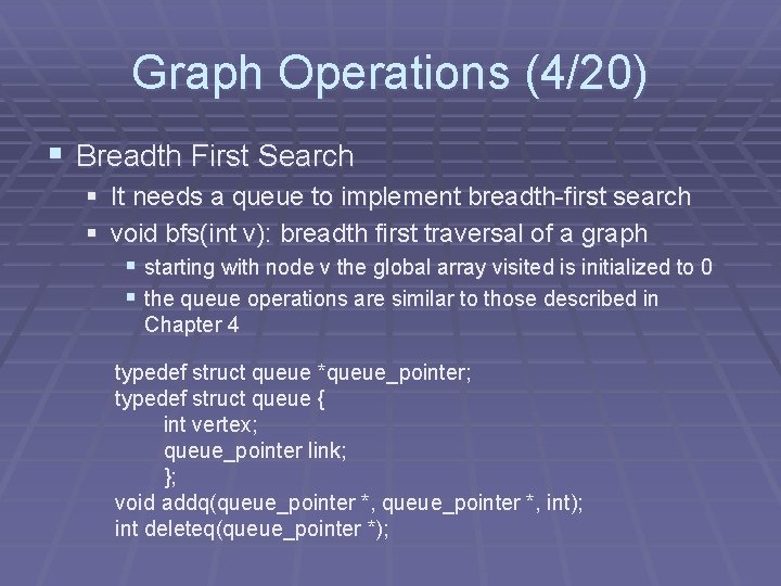
Graph Operations (4/20) § Breadth First Search § It needs a queue to implement breadth-first search § void bfs(int v): breadth first traversal of a graph § starting with node v the global array visited is initialized to 0 § the queue operations are similar to those described in Chapter 4 typedef struct queue *queue_pointer; typedef struct queue { int vertex; queue_pointer link; }; void addq(queue_pointer *, int); int deleteq(queue_pointer *);

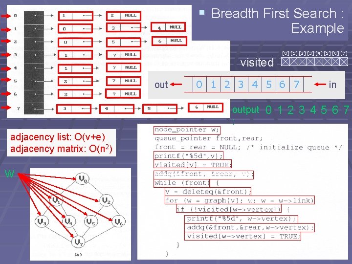
§ Breadth First Search : Example [0] [1] [2] [3] [4] [5] [6] [7] out visited : 0 1 2 3 4 5 6 7 output : adjacency list: O(v+e) adjacency matrix: O(n 2) w in 01234567

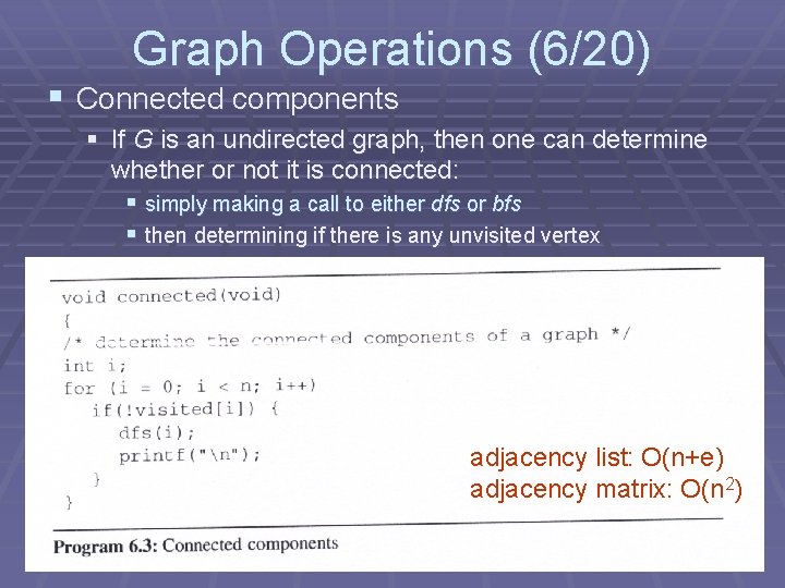
Graph Operations (6/20) § Connected components § If G is an undirected graph, then one can determine whether or not it is connected: § simply making a call to either dfs or bfs § then determining if there is any unvisited vertex adjacency list: O(n+e) adjacency matrix: O(n 2)

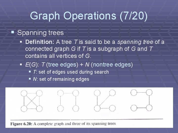
Graph Operations (7/20) § Spanning trees § Definition: A tree T is said to be a spanning tree of a connected graph G if T is a subgraph of G and T contains all vertices of G. § E(G): T (tree edges) + N (nontree edges) § T: set of edges used during search § N: set of remaining edges

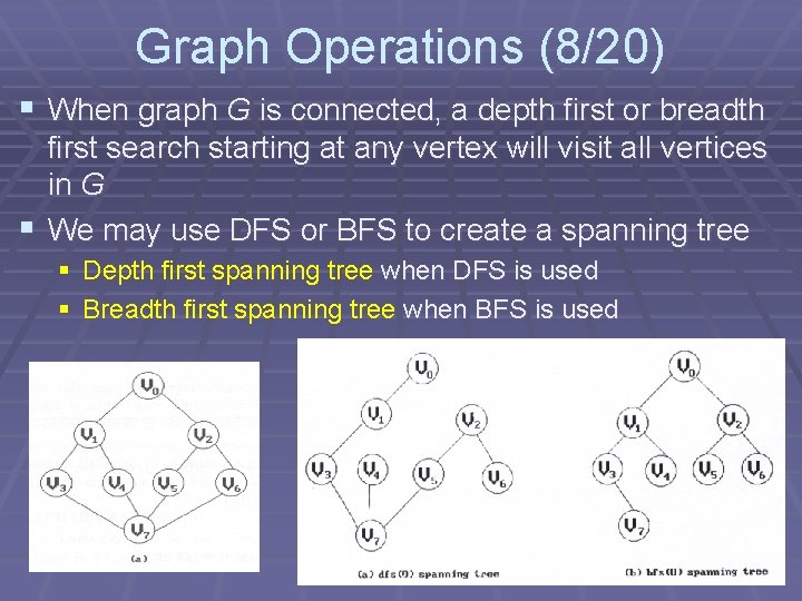
Graph Operations (8/20) § When graph G is connected, a depth first or breadth first search starting at any vertex will visit all vertices in G § We may use DFS or BFS to create a spanning tree § Depth first spanning tree when DFS is used § Breadth first spanning tree when BFS is used

Graph Operations (9/20) § Properties of spanning trees : § If a nontree edge (v, w) is introduced into any spanning tree T, then a cycle is formed. § A spanning tree is a minimal subgraph, G’, of G such that V(G’) = V(G) and G’ is connected. § We define a minimal subgraph as one with the fewest number of edge § A spanning tree has n-1 edges

Graph Operations (10/20) § Biconnected Graph & Articulation Points § § Assumption: G is an undirected, connected graph Definition: A vertex v of G is an articulation point iff the deletion of v, together with the deletion of all edges incident to v, leaves behind a graph that has at least two connected components. Definition: A biconnected graph is a connected graph that has no articulation points. Definition: A biconnected component of a connected graph G is a maximal biconnected subgraph H of G. § By maximal, we mean that G contains no other subgraph that is both biconnected and properly contains H.

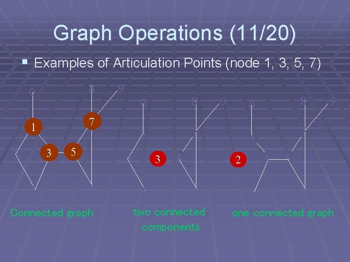
Graph Operations (11/20) § Examples of Articulation Points (node 1, 3, 5, 7) 8 0 3 4 0 8 1 7 7 1 2 9 5 3 2 6 Connected graph 4 5 9 0 8 1 7 2 6 two connected components 3 4 9 5 6 one connected graph

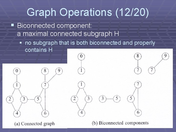
Graph Operations (12/20) § Biconnected component: a maximal connected subgraph H § no subgraph that is both biconnected and properly contains H

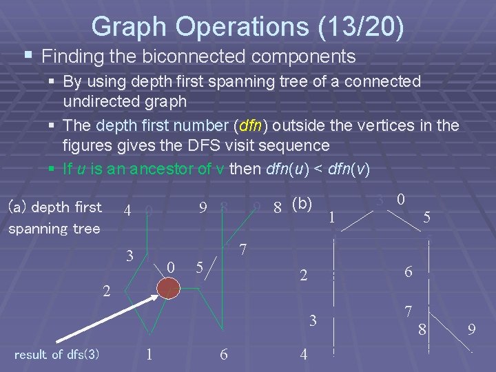
Graph Operations (13/20) § Finding the biconnected components § By using depth first spanning tree of a connected undirected graph § The depth first number (dfn) outside the vertices in the figures gives the DFS visit sequence § If u is an ancestor of v then dfn(u) < dfn(v) (a) depth first spanning tree 4 0 3 1 2 2 result of dfs(3) 9 8 4 1 9 8 (b) 7 7 0 3 5 5 2 6 6 3 4 1 4 3 0 5 5 2 6 6 1 7 7 8 9 0 9 8

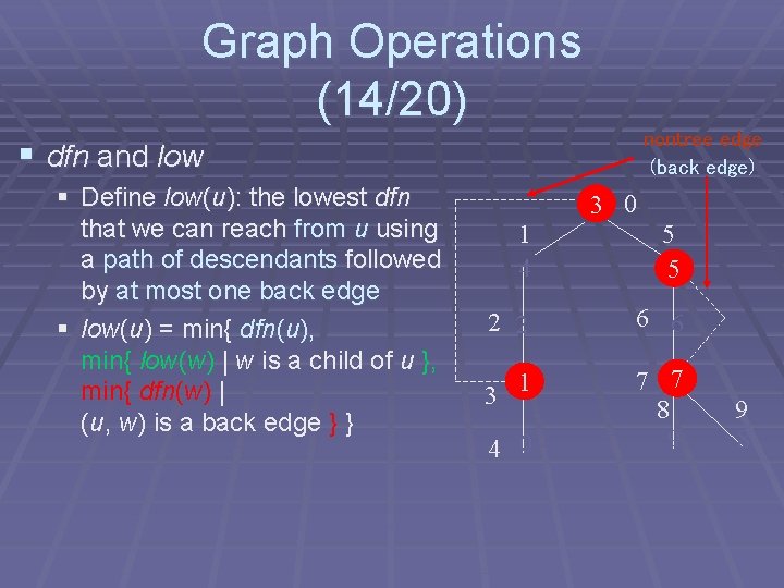
Graph Operations (14/20) nontree edge (back edge) § dfn and low § Define low(u): the lowest dfn that we can reach from u using a path of descendants followed by at most one back edge § low(u) = min{ dfn(u), min{ low(w) | w is a child of u }, min{ dfn(w) | (u, w) is a back edge } } 3 0 1 4 5 5 2 2 6 6 1 7 7 8 9 3 4 0 9 8

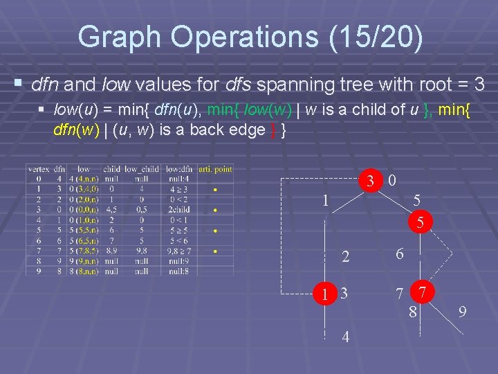
Graph Operations (15/20) § dfn and low values for dfs spanning tree with root = 3 § low(u) = min{ dfn(u), min{ low(w) | w is a child of u }, min{ dfn(w) | (u ( , w) is a back edge } } 3 0 1 4 5 5 2 2 6 6 1 3 7 7 8 9 0 4 9 8

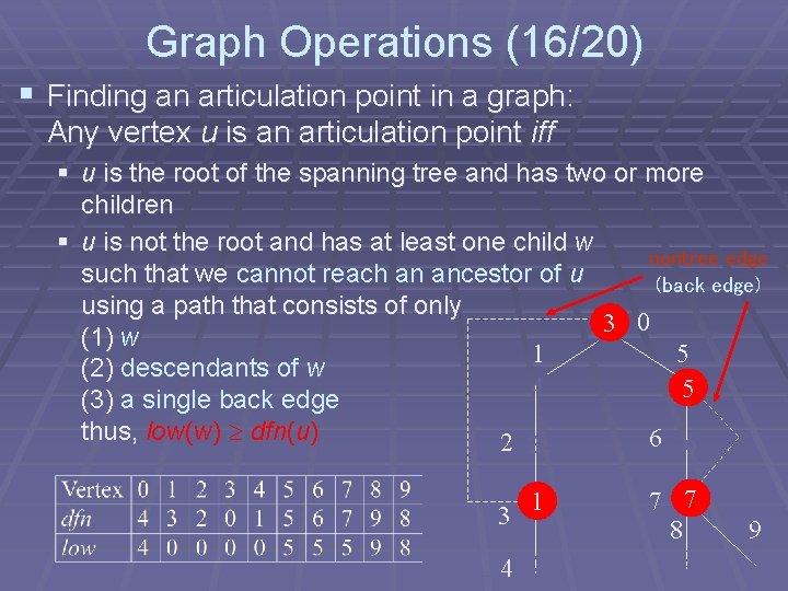
Graph Operations (16/20) § Finding an articulation point in a graph: Any vertex u is an articulation point iff § u is the root of the spanning tree and has two or more children § u is not the root and has at least one child w nontree edge such that we cannot reach an ancestor of u (back edge) using a path that consists of only 3 0 (1) w 1 5 (2) descendants of w 4 5 (3) a single back edge thus, low(w) dfn(u) 6 6 2 2 3 1 4 0 7 7 8 9 9 8

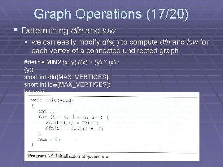
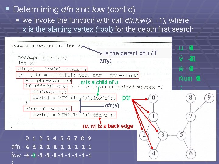
Graph Operations (17/20) § Determining dfn and low § we can easily modify dfs( ) to compute dfn and low for each vertex of a connected undirected graph #define MIN 2 (x, y) ((x) < (y) ? (x) : (y)) short int dfn[MAX_VERTICES]; short int low[MAX_VERTICES]; int num;

§ Determining dfn and low (cont’d) § we invoke the function with call dfnlow(x, -1), where x is the starting vertex (root) for the depth first search v is the parent of u (if any) w is a child of u ptr dfn(u) (u, w) is a back edge 0 1 2 3 4 5 6 7 8 9 dfn -1 4 -1 3 -1 2 -1 0 -1 1 -1 -1 -1 : low -1 4 -1 3 -1 0 2 -1 0 -1 1 -1 -1 -1 : u 0 3 4 2 1 : 3 4 1 2 v -1 : w 0 4 2 1 3 : num 4 2 3 0 1 5 :

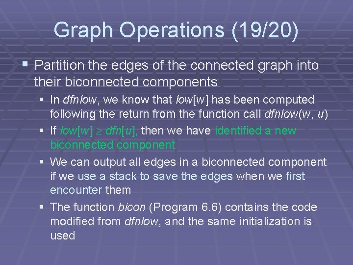
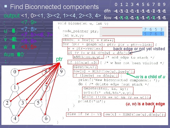
Graph Operations (19/20) § Partition the edges of the connected graph into their biconnected components § In dfnlow, we know that low[w] has been computed following the return from the function call dfnlow(w, u) § If low[w] dfn[u], then we have identified a new biconnected component § We can output all edges in a biconnected component if we use a stack to save the edges when we first encounter them § The function bicon (Program 6. 6) contains the code modified from dfnlow, and the same initialization is used

§ Find Biconnected components output <1, 0><1, 3><2, 1><4, 2><3, 4> <7, 9> : u 3 0 <7, 8> 1 2 4 9 8 7 6 5 <7, 5><6, 7> : -1 1 <5, 6> 2 4 7 6 5 3 v -1 : w 7 0 <3, 5> 1 4 2 9 8 5 6 3 : num 10 0 1 2 3 4 5 6 7 8 9 ptr : 0 1 2 3 4 5 6 7 8 9 dfn -1 0 -1 1 -1 7 -1 4 -1 3 -1 2 -1 5 -1 6 -1 9 -1 8 : low -1 7 4 -1 3 -1 0 2 0 -1 0 5 -1 6 -1 5 5 -1 9 -1 8 1 -1 : 1 2 7 6 5 4 3 0 7 3 9 8 5 1 2 6 4 5 back edge or not yet visited w is a child of u (u, w) is a back edge

Minimum Cost Spanning Trees (1/7) § Introduction § The cost of a spanning tree of a weighted, undirected graph is the sum of the costs (weights) of the edges in the spanning tree. § A minimum-cost spanning tree is a spanning tree of least cost. § Three different algorithms can be used to obtain a minimum cost spanning tree. § Kruskal’s algorithm § Prim’s algorithm § Sollin’s algorithm § All the three use a design strategy called the greedy method

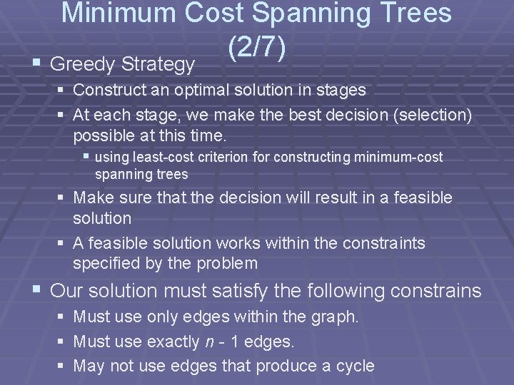
Minimum Cost Spanning Trees (2/7) § Greedy Strategy § Construct an optimal solution in stages § At each stage, we make the best decision (selection) possible at this time. § using least-cost criterion for constructing minimum-cost spanning trees § Make sure that the decision will result in a feasible solution § A feasible solution works within the constraints specified by the problem § Our solution must satisfy the following constrains § Must use only edges within the graph. § Must use exactly n - 1 edges. § May not use edges that produce a cycle

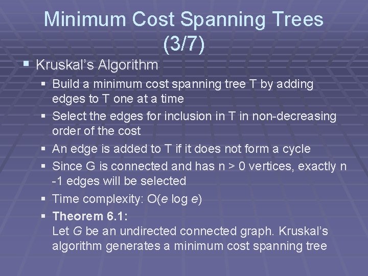
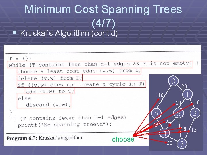
Minimum Cost Spanning Trees (3/7) § Kruskal’s Algorithm § Build a minimum cost spanning tree T by adding edges to T one at a time § Select the edges for inclusion in T in non-decreasing order of the cost § An edge is added to T if it does not form a cycle § Since G is connected and has n > 0 vertices, exactly n -1 edges will be selected § Time complexity: O(e log e) § Theorem 6. 1: Let G be an undirected connected graph. Kruskal’s algorithm generates a minimum cost spanning tree

Minimum Cost Spanning Trees (4/7) § Kruskal’s Algorithm (cont’d) 0 28 1 10 5 25 choose 14 16 6 2 24 4 22 18 12 3

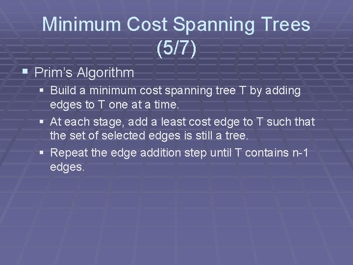
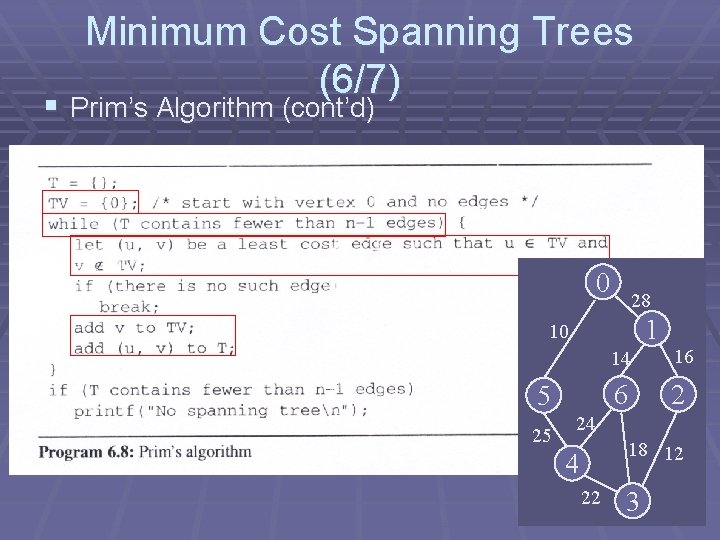
Minimum Cost Spanning Trees (5/7) § Prim’s Algorithm § Build a minimum cost spanning tree T by adding edges to T one at a time. § At each stage, add a least cost edge to T such that the set of selected edges is still a tree. § Repeat the edge addition step until T contains n-1 edges.

Minimum Cost Spanning Trees (6/7) § Prim’s Algorithm (cont’d) 0 28 1 10 5 25 14 16 6 2 24 18 12 4 22 3

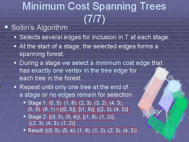
Minimum Cost Spanning Trees (7/7) § Sollin’s Algorithm § Selects several edges for inclusion in T at each stage. § At the start of a stage, the selected edges forms a spanning forest. § During a stage we select a minimum cost edge that has exactly one vertex in the tree edge for 0 28 each tree in the forest. 10 1 § Repeat until only one tree at the end of 16 14 a stage or no edges remain for selection. § Stage 1: (0, 5), (1, 6), (2, 3), (3, 2), (4, 3), 6 2 5 (5, 0), (6, 1) {(0, 5)}, {(1, 6)}, {(2, 3), (4, 3)} 25 § Stage 2: {(0, 5), (5, 4)}, {(1, 6), (1, 2)}, {(2, 3), (4, 3), (1, 2)} § Result: {(0, 5), (5, 4), (1, 6), (1, 2), (2, 3), (4, 3)} 24 18 12 4 22 3