Data Mining Toon Calders Why Data mining l

Data Mining Toon Calders

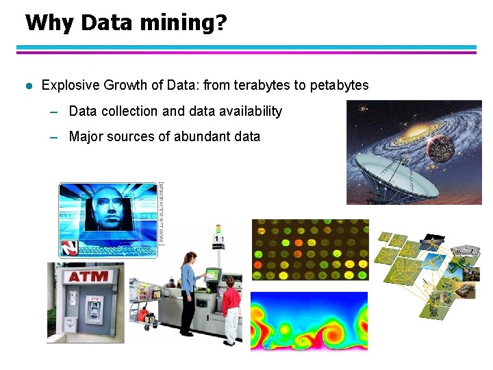
Why Data mining? l Explosive Growth of Data: from terabytes to petabytes – Data collection and data availability – Major sources of abundant data

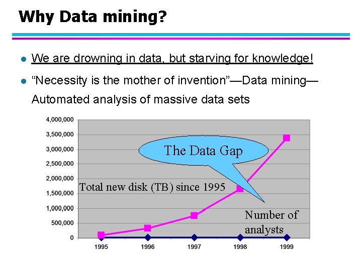
Why Data mining? l We are drowning in data, but starving for knowledge! l “Necessity is the mother of invention”—Data mining— Automated analysis of massive data sets The Data Gap Total new disk (TB) since 1995 Number of analysts

What Is Data Mining? l Data mining (knowledge discovery from data) – Extraction of interesting (non-trivial, implicit, previously unknown and potentially useful) patterns or knowledge from huge amount of data l Alternative names – Knowledge discovery (mining) in databases (KDD), knowledge extraction, data/pattern analysis, data archeology, data dredging, information harvesting, business intelligence, etc.

Current Applications l Data analysis and decision support – Market analysis and management – Risk analysis and management – Fraud detection and detection of unusual patterns (outliers) l Other Applications – Text mining (news group, email, documents) and Web mining – Stream data mining – Bioinformatics and bio-data analysis

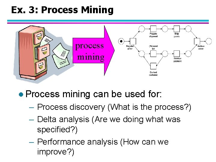
Ex. 3: Process Mining process mining l Process mining can be used for: – Process discovery (What is the process? ) – Delta analysis (Are we doing what was specified? ) – Performance analysis (How can we improve? )

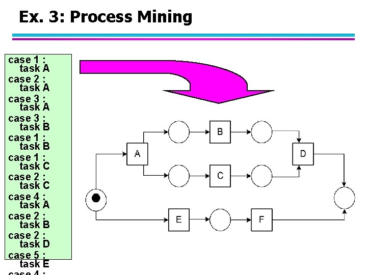
Ex. 3: Process Mining case 1 : task A case 2 : task A case 3 : task B case 1 : task C case 2 : task C case 4 : task A case 2 : task B case 2 : task D case 5 : task E

Data Mining Tasks l Previous lectures: – Classification [Predictive] – Clustering [Descriptive] l This lecture: – Association Rule Discovery [Descriptive] – Sequential Pattern Discovery [Descriptive] l Other techniques: – Regression [Predictive] – Deviation Detection [Predictive]

Outline of today’s lecture l Association Rule Mining – Frequent itemsets and association rules – Algorithms: Apriori and Eclat l Sequential Pattern Mining – Mining frequent episodes – Algorithms: Win. Epi and Min. Epi l Other types of patterns – strings, graphs, … – process mining

Association Rule Mining l Definition – Frequent itemsets – Association rules l Frequent itemset mining – breadth-first Apriori – depth-first Eclat l Association Rule Mining

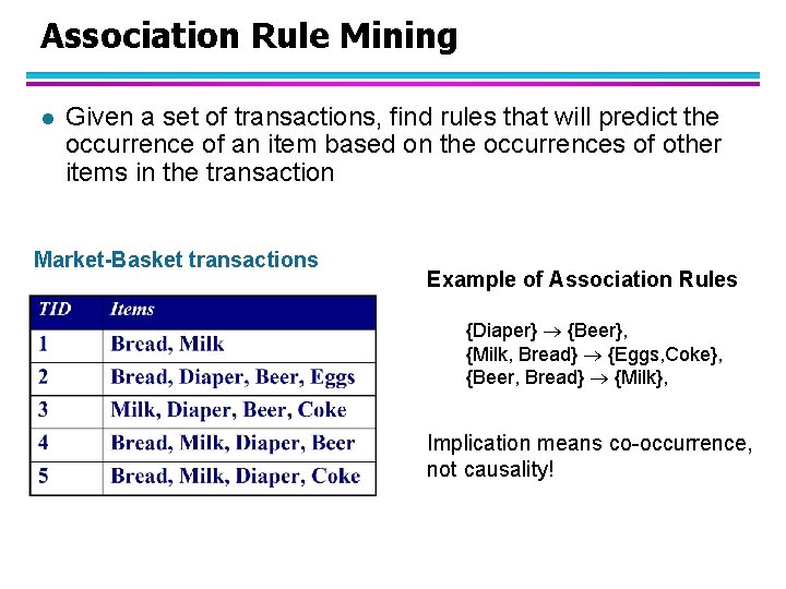
Association Rule Mining l Given a set of transactions, find rules that will predict the occurrence of an item based on the occurrences of other items in the transaction Market-Basket transactions Example of Association Rules {Diaper} {Beer}, {Milk, Bread} {Eggs, Coke}, {Beer, Bread} {Milk}, Implication means co-occurrence, not causality!

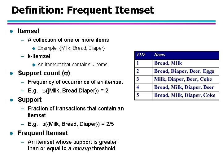
Definition: Frequent Itemset l Itemset – A collection of one or more items u Example: {Milk, Bread, Diaper} – k-itemset u l An itemset that contains k items Support count ( ) – Frequency of occurrence of an itemset – E. g. ({Milk, Bread, Diaper}) = 2 l Support – Fraction of transactions that contain an itemset – E. g. s({Milk, Bread, Diaper}) = 2/5 l Frequent Itemset – An itemset whose support is greater than or equal to a minsup threshold

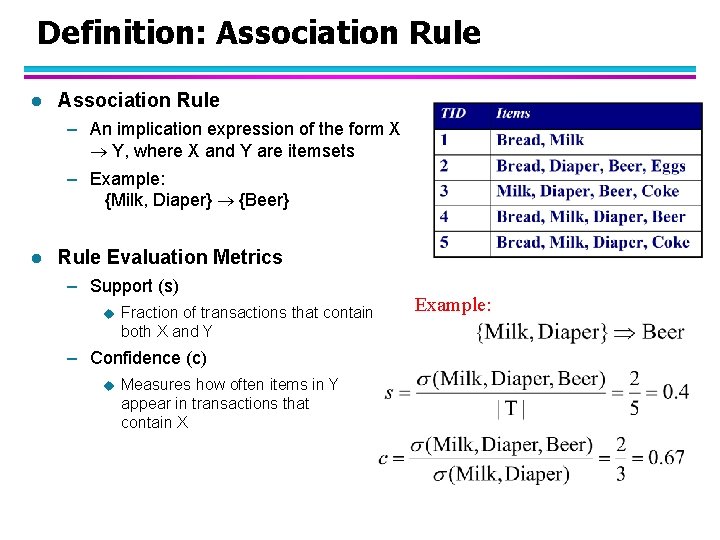
Definition: Association Rule l Association Rule – An implication expression of the form X Y, where X and Y are itemsets – Example: {Milk, Diaper} {Beer} l Rule Evaluation Metrics – Support (s) u Fraction of transactions that contain both X and Y – Confidence (c) u Measures how often items in Y appear in transactions that contain X Example:

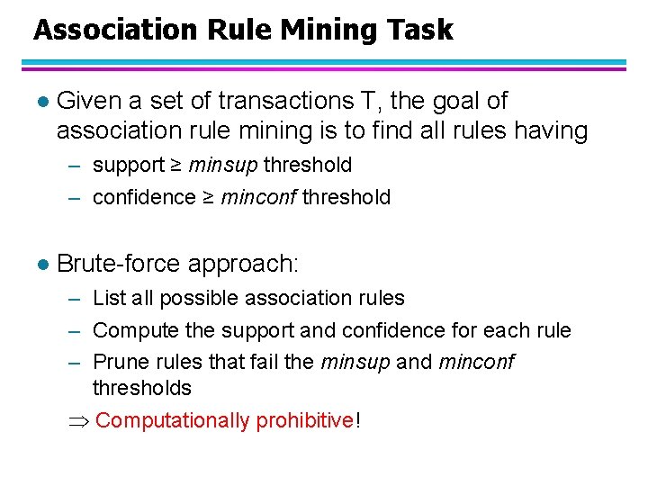
Association Rule Mining Task l Given a set of transactions T, the goal of association rule mining is to find all rules having – support ≥ minsup threshold – confidence ≥ minconf threshold l Brute-force approach: – List all possible association rules – Compute the support and confidence for each rule – Prune rules that fail the minsup and minconf thresholds Computationally prohibitive!

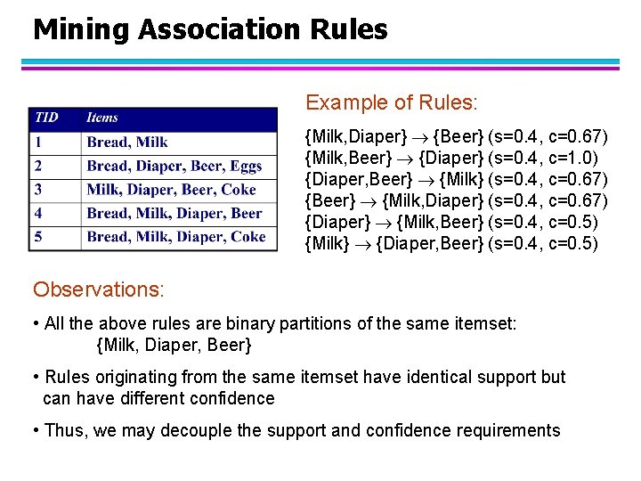
Mining Association Rules Example of Rules: {Milk, Diaper} {Beer} (s=0. 4, c=0. 67) {Milk, Beer} {Diaper} (s=0. 4, c=1. 0) {Diaper, Beer} {Milk} (s=0. 4, c=0. 67) {Beer} {Milk, Diaper} (s=0. 4, c=0. 67) {Diaper} {Milk, Beer} (s=0. 4, c=0. 5) {Milk} {Diaper, Beer} (s=0. 4, c=0. 5) Observations: • All the above rules are binary partitions of the same itemset: {Milk, Diaper, Beer} • Rules originating from the same itemset have identical support but can have different confidence • Thus, we may decouple the support and confidence requirements

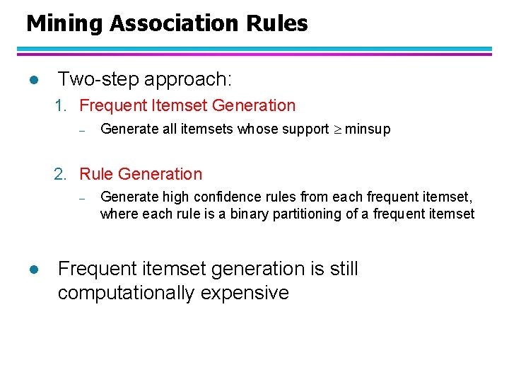
Mining Association Rules l Two-step approach: 1. Frequent Itemset Generation – Generate all itemsets whose support minsup 2. Rule Generation – l Generate high confidence rules from each frequent itemset, where each rule is a binary partitioning of a frequent itemset Frequent itemset generation is still computationally expensive

Association Rule Mining l Definition – Frequent itemsets – Association rules l Frequent itemset mining – breadth-first Apriori – depth-first Eclat l Association Rule Mining

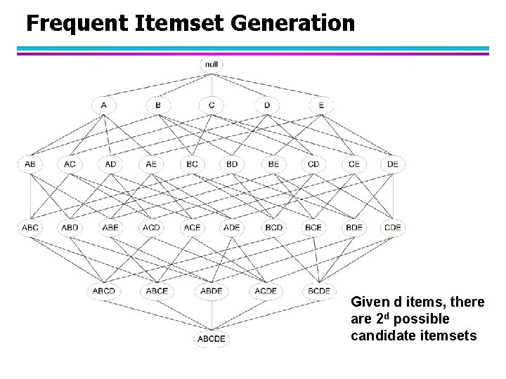
Frequent Itemset Generation Given d items, there are 2 d possible candidate itemsets

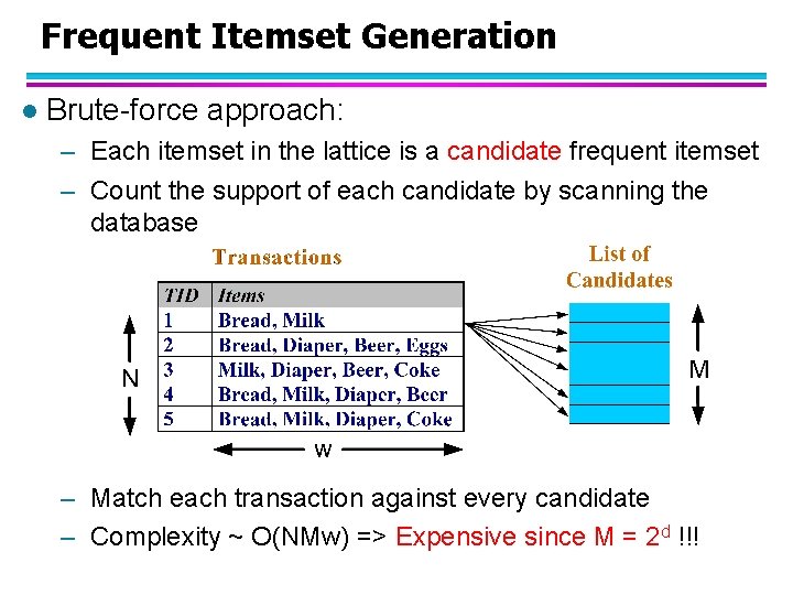
Frequent Itemset Generation l Brute-force approach: – Each itemset in the lattice is a candidate frequent itemset – Count the support of each candidate by scanning the database – Match each transaction against every candidate – Complexity ~ O(NMw) => Expensive since M = 2 d !!!

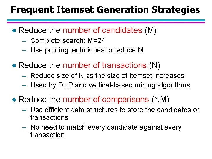
Frequent Itemset Generation Strategies l Reduce the number of candidates (M) – Complete search: M=2 d – Use pruning techniques to reduce M l Reduce the number of transactions (N) – Reduce size of N as the size of itemset increases – Used by DHP and vertical-based mining algorithms l Reduce the number of comparisons (NM) – Use efficient data structures to store the candidates or transactions – No need to match every candidate against every transaction

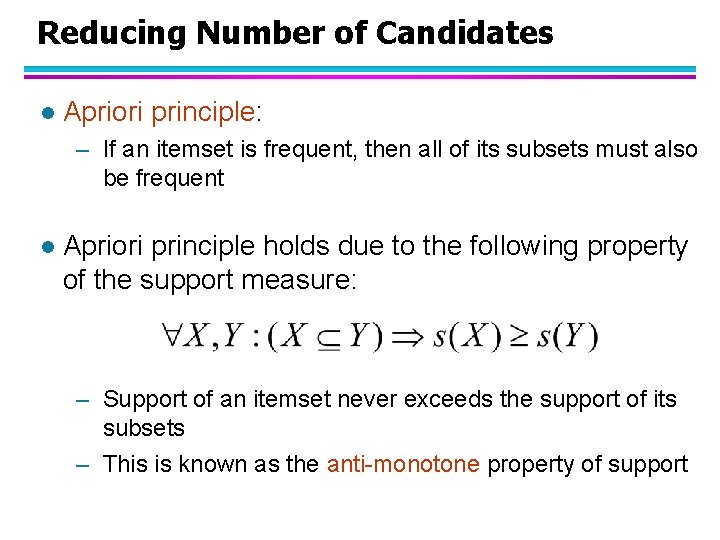
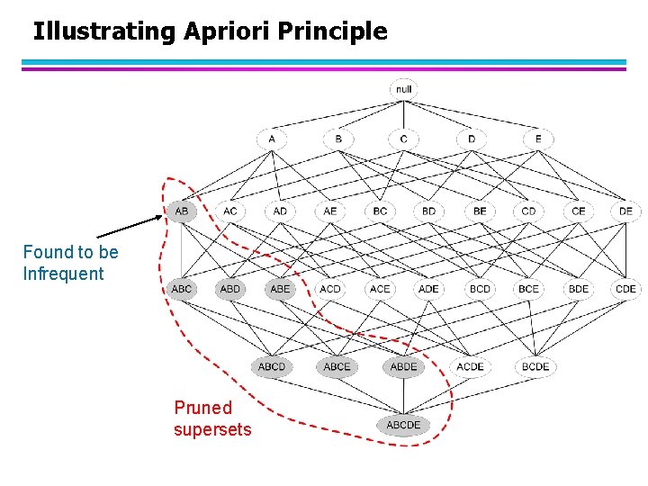
Reducing Number of Candidates l Apriori principle: – If an itemset is frequent, then all of its subsets must also be frequent l Apriori principle holds due to the following property of the support measure: – Support of an itemset never exceeds the support of its subsets – This is known as the anti-monotone property of support

Illustrating Apriori Principle Found to be Infrequent Pruned supersets

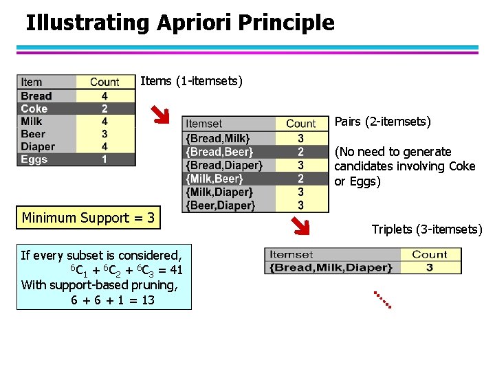
Illustrating Apriori Principle Items (1 -itemsets) Pairs (2 -itemsets) (No need to generate candidates involving Coke or Eggs) Minimum Support = 3 If every subset is considered, 6 C + 6 C = 41 1 2 3 With support-based pruning, 6 + 1 = 13 Triplets (3 -itemsets)

Association Rule Mining l Definition – Frequent itemsets – Association rules l Frequent itemset mining – breadth-first Apriori – depth-first Eclat l Association Rule Mining

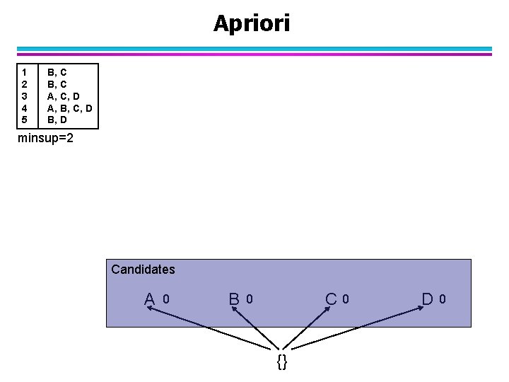
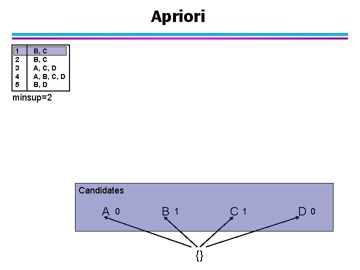
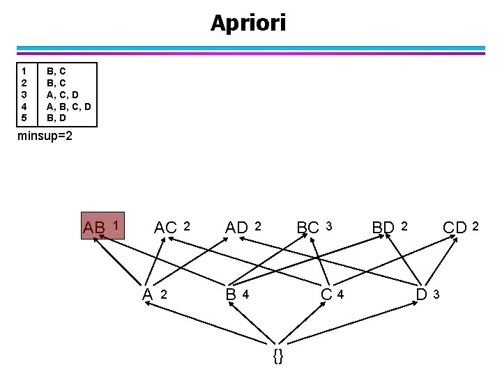
Apriori 1 2 3 4 5 B, C A, C, D A, B, C, D B, D minsup=2 Candidates A 0 B C 0 0 {} D 0

Apriori 1 2 3 4 5 B, C A, C, D A, B, C, D B, D minsup=2 Candidates A 0 B C 1 1 {} D 0

Apriori 1 2 3 4 5 B, C A, C, D A, B, C, D B, D minsup=2 Candidates A 0 B C 2 2 {} D 0

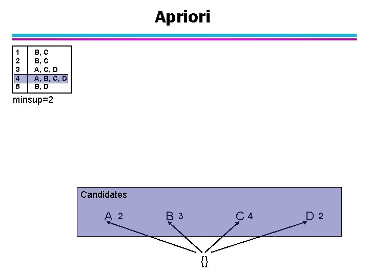
Apriori 1 2 3 4 5 B, C A, C, D A, B, C, D B, D minsup=2 Candidates A 1 B C 3 2 {} D 1

Apriori 1 2 3 4 5 B, C A, C, D A, B, C, D B, D minsup=2 Candidates A 2 B C 4 3 {} D 2

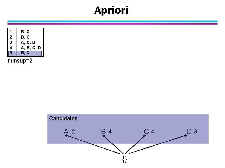
Apriori 1 2 3 4 5 B, C A, C, D A, B, C, D B, D minsup=2 Candidates A 2 B C 4 4 {} D 3

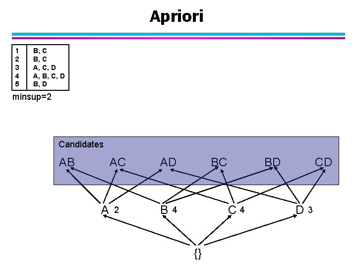
Apriori 1 2 3 4 5 B, C A, C, D A, B, C, D B, D minsup=2 Candidates AB AC A 2 AD B BC BD C 4 4 {} CD D 3

Apriori 1 2 3 4 5 B, C A, C, D A, B, C, D B, D minsup=2 AB AC 1 A 2 2 AD B BC 2 3 C 4 4 {} BD CD 2 2 D 3

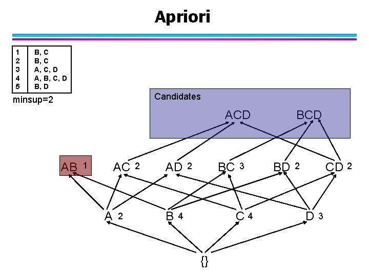
Apriori 1 2 3 4 5 B, C A, C, D A, B, C, D B, D Candidates minsup=2 ACD AB AC 1 A 2 2 AD B BC 2 3 C 4 4 {} BCD BD CD 2 2 D 3

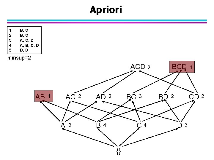
Apriori 1 2 3 4 5 B, C A, C, D A, B, C, D B, D minsup=2 ACD 2 AB AC 1 A 2 2 AD B BC 2 3 C 4 4 {} BD BCD 1 2 CD 2 D 3

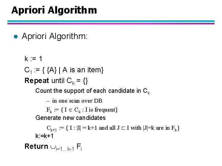
Apriori Algorithm l Apriori Algorithm: k : = 1 C 1 : = { {A} | A is an item} Repeat until Ck = {} Count the support of each candidate in Ck – in one scan over DB Fk : = { I Ck : I is frequent} Generate new candidates Ck+1 : = { I : |I| = k+1 and all J I with |J|=k are in Fk} k: =k+1 Return i=1…k-1 Fi

Association Rule Mining l Definition – Frequent itemsets – Association rules l Frequent itemset mining – breadth-first Apriori – depth-first Eclat l Association Rule Mining

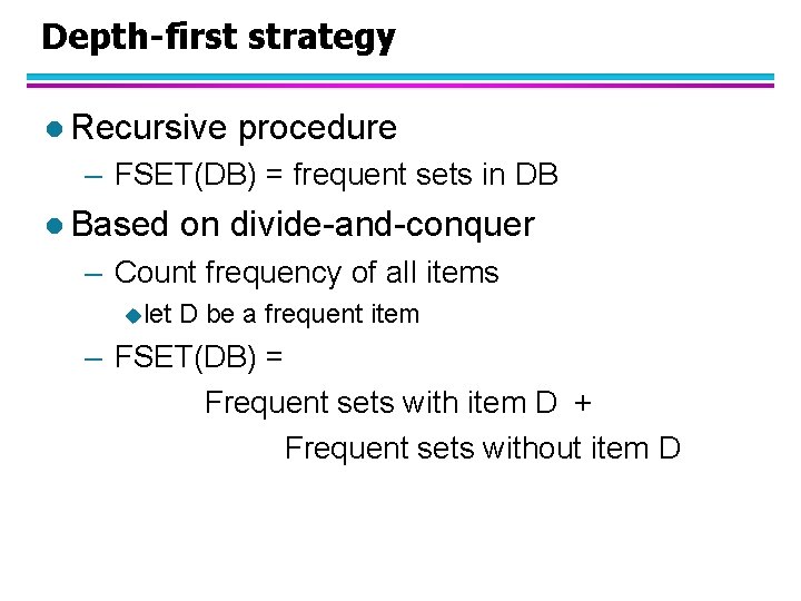
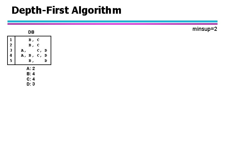
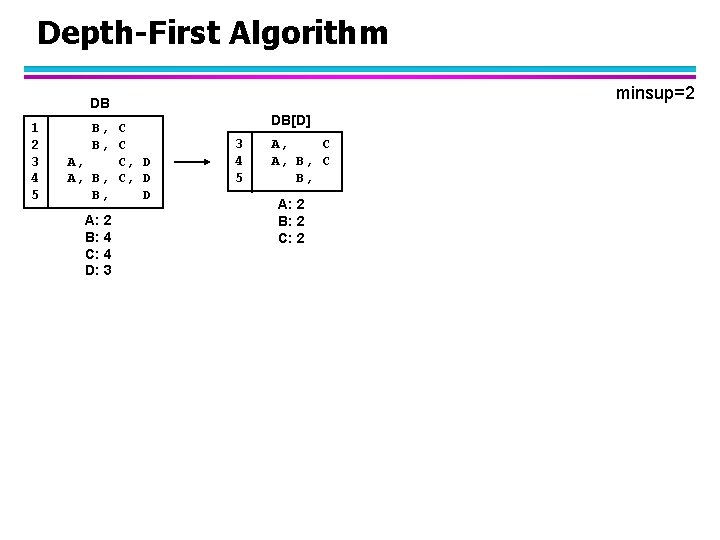
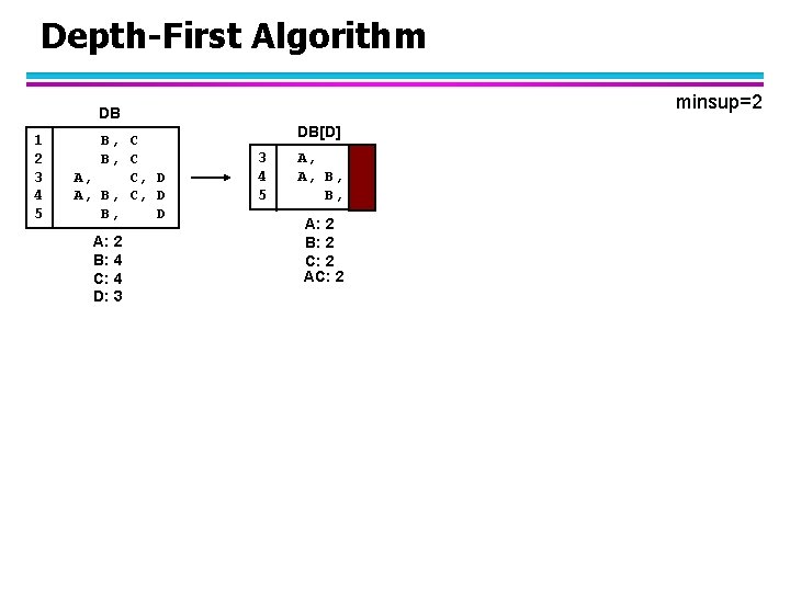
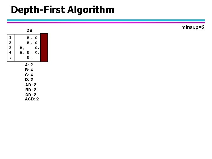
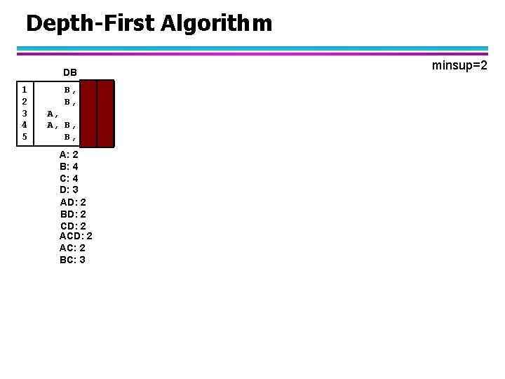
Depth-first strategy l Recursive procedure – FSET(DB) = frequent sets in DB l Based on divide-and-conquer – Count frequency of all items ulet D be a frequent item – FSET(DB) = Frequent sets with item D + Frequent sets without item D

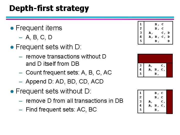
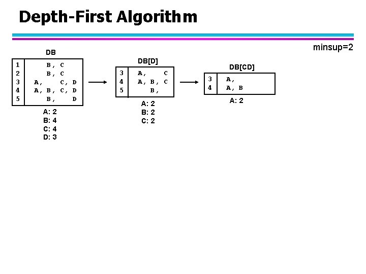
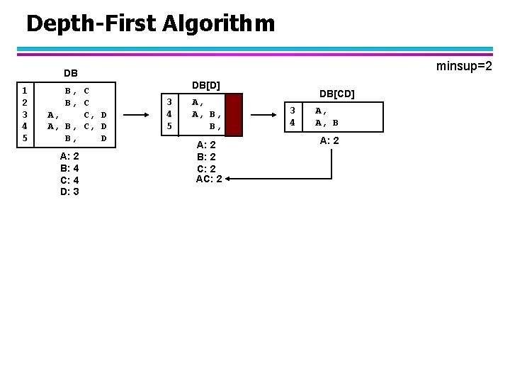
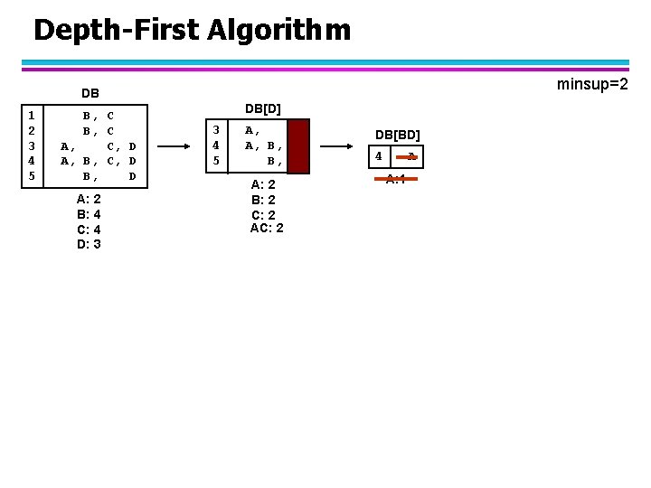
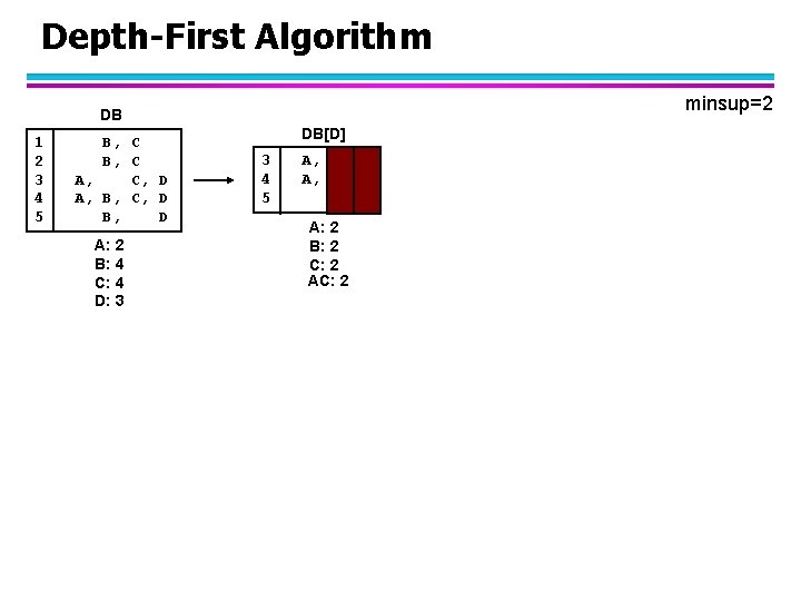
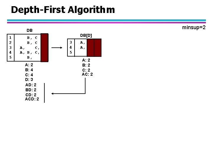
Depth-first strategy l Frequent items – A, B, C, D l Frequent sets with D: – remove transactions without D and D itself from DB – Count frequent sets: A, B, C, AC – Append D: AD, BD, CD, ACD l Frequent sets without D: – remove D from all transactions in DB – Find frequent sets: AC, BC 1 2 3 4 5 B, C A, C, D A, B, C, D B, D 1 2 3 4 5 B, C A, C, D A, B, C, D B, D

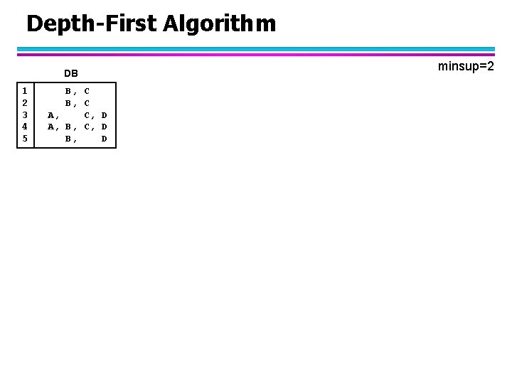
Depth-First Algorithm DB 1 2 3 4 5 B, C A, C, D A, B, C, D B, D minsup=2

Depth-First Algorithm DB 1 2 3 4 5 B, C A, C, D A, B, C, D B, D A: 2 B: 4 C: 4 D: 3 minsup=2

Depth-First Algorithm minsup=2 DB 1 2 3 4 5 B, C A, C, D A, B, C, D B, D A: 2 B: 4 C: 4 D: 3 DB[D] 3 4 5 A, C A, B, C B, A: 2 B: 2 C: 2

Depth-First Algorithm minsup=2 DB 1 2 3 4 5 B, C A, C, D A, B, C, D B, D A: 2 B: 4 C: 4 D: 3 DB[D] 3 4 5 A, C A, B, C B, A: 2 B: 2 C: 2 DB[CD] 3 4 A, A, B A: 2

Depth-First Algorithm minsup=2 DB 1 2 3 4 5 B, C A, C, D A, B, C, D B, D A: 2 B: 4 C: 4 D: 3 DB[D] 3 4 5 A, C A, B, C B, A: 2 B: 2 C: 2 AC: 2 DB[CD] 3 4 A, A, B A: 2

Depth-First Algorithm minsup=2 DB 1 2 3 4 5 B, C A, C, D A, B, C, D B, D A: 2 B: 4 C: 4 D: 3 DB[D] 3 4 5 A, C A, B, C B, A: 2 B: 2 C: 2 AC: 2

Depth-First Algorithm minsup=2 DB 1 2 3 4 5 B, C A, C, D A, B, C, D B, D A: 2 B: 4 C: 4 D: 3 DB[D] 3 4 5 A, C A, B, C B, A: 2 B: 2 C: 2 AC: 2 DB[BD] 4 A A: 1

Depth-First Algorithm minsup=2 DB 1 2 3 4 5 B, C A, C, D A, B, C, D B, D A: 2 B: 4 C: 4 D: 3 DB[D] 3 4 5 A, C A, B, C B, A: 2 B: 2 C: 2 AC: 2

Depth-First Algorithm minsup=2 DB 1 2 3 4 5 B, C A, C, D A, B, C, D B, D A: 2 B: 4 C: 4 D: 3 AD: 2 BD: 2 CD: 2 ACD: 2 DB[D] 3 4 5 A, C A, B, C B, A: 2 B: 2 C: 2 AC: 2

Depth-First Algorithm DB 1 2 3 4 5 B, C A, C, D A, B, C, D B, D A: 2 B: 4 C: 4 D: 3 AD: 2 BD: 2 CD: 2 ACD: 2 minsup=2

Depth-First Algorithm DB[C] DB 1 2 3 4 5 B, C A, C, D A, B, C, D B, D A: 2 B: 4 C: 4 D: 3 AD: 2 BD: 2 CD: 2 ACD: 2 1 2 3 4 B B A A, B A: 2 B: 3 minsup=2

Depth-First Algorithm DB[C] DB 1 2 3 4 5 B, C A, C, D A, B, C, D B, D A: 2 B: 4 C: 4 D: 3 AD: 2 BD: 2 CD: 2 ACD: 2 1 2 3 4 B B A A, B A: 2 B: 3 DB[BC] 1 2 4 A A: 1 minsup=2

Depth-First Algorithm DB[C] DB 1 2 3 4 5 B, C A, C, D A, B, C, D B, D A: 2 B: 4 C: 4 D: 3 AD: 2 BD: 2 CD: 2 ACD: 2 1 2 3 4 B B A A, B A: 2 B: 3 minsup=2

Depth-First Algorithm DB[C] DB 1 2 3 4 5 B, C A, C, D A, B, C, D B, D A: 2 B: 4 C: 4 D: 3 AD: 2 BD: 2 CD: 2 AC: 2 BC: 3 1 2 3 4 B B A A, B A: 2 B: 3 minsup=2

Depth-First Algorithm DB 1 2 3 4 5 B, C A, C, D A, B, C, D B, D A: 2 B: 4 C: 4 D: 3 AD: 2 BD: 2 CD: 2 AC: 2 BC: 3 minsup=2

Depth-First Algorithm DB[B] DB 1 2 3 4 5 B, C A, C, D A, B, C, D B, D A: 2 B: 4 C: 4 D: 3 AD: 2 BD: 2 CD: 2 AC: 2 BC: 3 1 2 4 5 A A: 1 minsup=2

Depth-First Algorithm DB 1 2 3 4 5 B, C A, C, D A, B, C, D B, D A: 2 B: 4 C: 4 D: 3 AD: 2 BD: 2 CD: 2 AC: 2 BC: 3 minsup=2

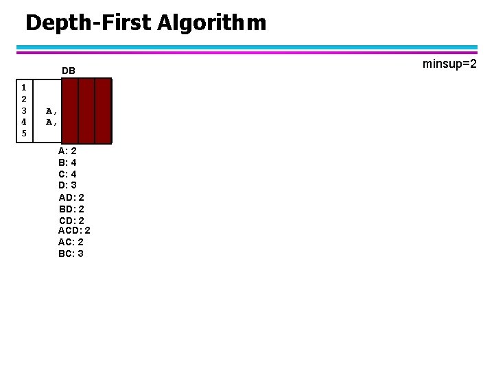
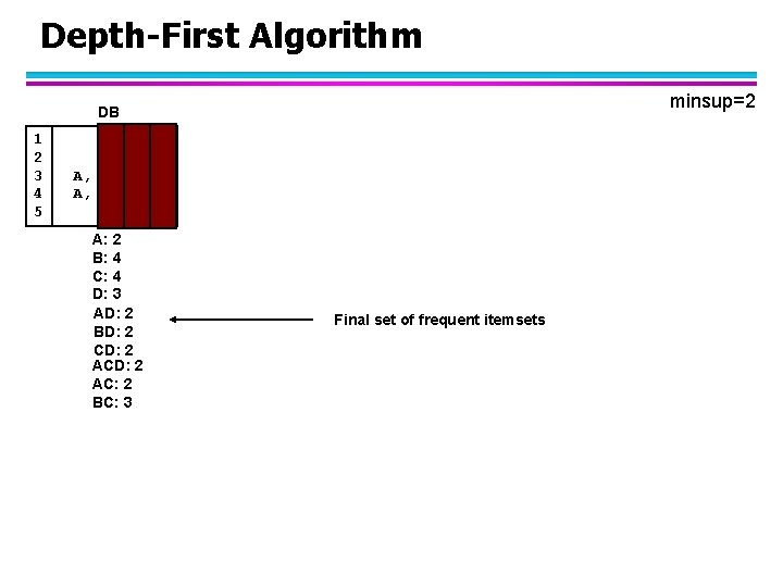
Depth-First Algorithm minsup=2 DB 1 2 3 4 5 B, C A, C, D A, B, C, D B, D A: 2 B: 4 C: 4 D: 3 AD: 2 BD: 2 CD: 2 AC: 2 BC: 3 Final set of frequent itemsets

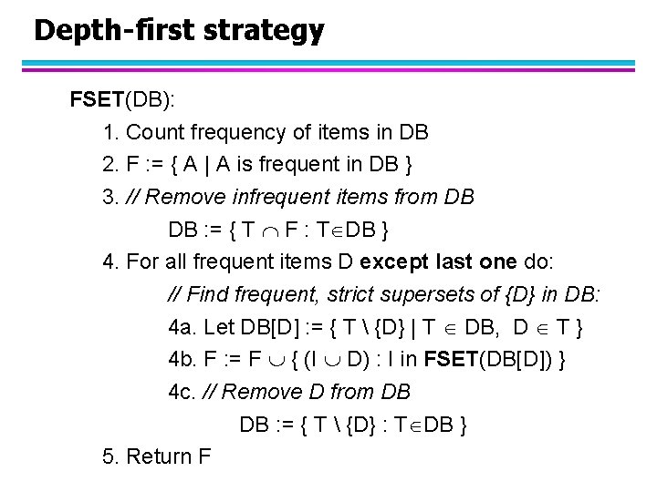
Depth-first strategy FSET(DB): 1. Count frequency of items in DB 2. F : = { A | A is frequent in DB } 3. // Remove infrequent items from DB DB : = { T F : T DB } 4. For all frequent items D except last one do: // Find frequent, strict supersets of {D} in DB: 4 a. Let DB[D] : = { T {D} | T DB, D T } 4 b. F : = F { (I D) : I in FSET(DB[D]) } 4 c. // Remove D from DB DB : = { T {D} : T DB } 5. Return F

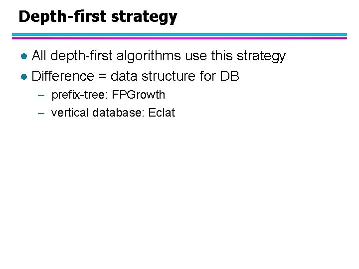
Depth-first strategy All depth-first algorithms use this strategy l Difference = data structure for DB l – prefix-tree: FPGrowth – vertical database: Eclat

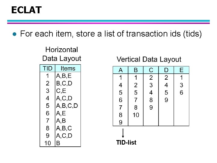
ECLAT l For each item, store a list of transaction ids (tids) TID-list

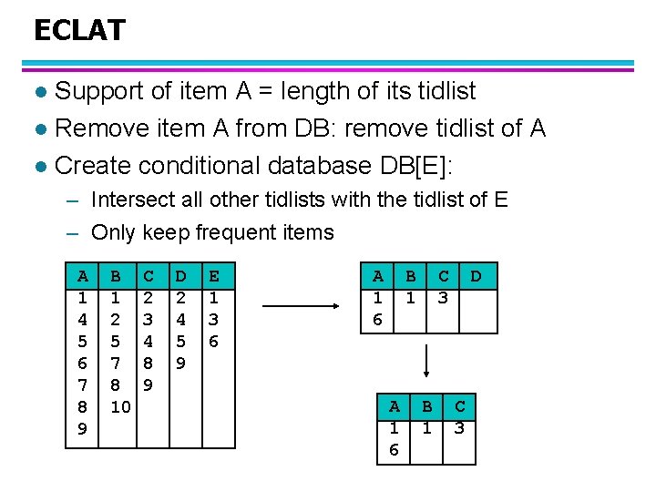
ECLAT Support of item A = length of its tidlist l Remove item A from DB: remove tidlist of A l Create conditional database DB[E]: l – Intersect all other tidlists with the tidlist of E – Only keep frequent items A 1 4 5 6 7 8 9 B 1 2 5 7 8 10 C 2 3 4 8 9 D 2 4 5 9 E 1 3 6 A 1 6 B 1 A 1 6 C 3 B 1 D C 3

Association Rule Mining l Definition – Frequent itemsets – Association rules l Frequent itemset mining – breadth-first Apriori – depth-first Eclat l Association Rule Mining

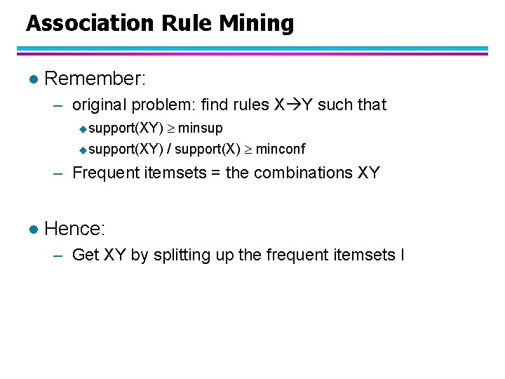
Association Rule Mining l Remember: – original problem: find rules X Y such that usupport(XY) minsup / support(X) minconf – Frequent itemsets = the combinations XY l Hence: – Get XY by splitting up the frequent itemsets I

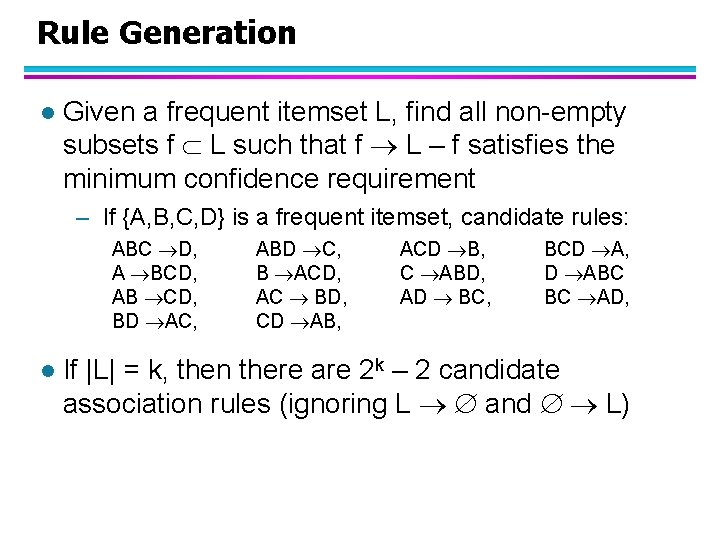
Rule Generation l Given a frequent itemset L, find all non-empty subsets f L such that f L – f satisfies the minimum confidence requirement – If {A, B, C, D} is a frequent itemset, candidate rules: ABC D, A BCD, AB CD, BD AC, l ABD C, B ACD, AC BD, CD AB, ACD B, C ABD, AD BC, BCD A, D ABC BC AD, If |L| = k, then there are 2 k – 2 candidate association rules (ignoring L and L)

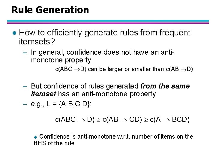
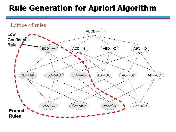
Rule Generation l How to efficiently generate rules from frequent itemsets? – In general, confidence does not have an antimonotone property c(ABC D) can be larger or smaller than c(AB D) – But confidence of rules generated from the same itemset has an anti-monotone property – e. g. , L = {A, B, C, D}: c(ABC D) c(AB CD) c(A BCD) Confidence is anti-monotone w. r. t. number of items on the RHS of the rule u

Rule Generation for Apriori Algorithm Lattice of rules Low Confidence Rule Pruned Rules

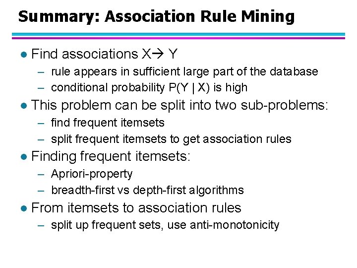
Summary: Association Rule Mining l Find associations X Y – rule appears in sufficient large part of the database – conditional probability P(Y | X) is high l This problem can be split into two sub-problems: – find frequent itemsets – split frequent itemsets to get association rules l Finding frequent itemsets: – Apriori-property – breadth-first vs depth-first algorithms l From itemsets to association rules – split up frequent sets, use anti-monotonicity

Outline l Association Rule Mining – Frequent itemsets and association rules – Algorithms: Apriori and Eclat l Sequential Pattern Mining – Mining frequent episodes – Algorithms: Win. Epi and Min. Epi l Other types of patterns – strings, graphs, … – process mining

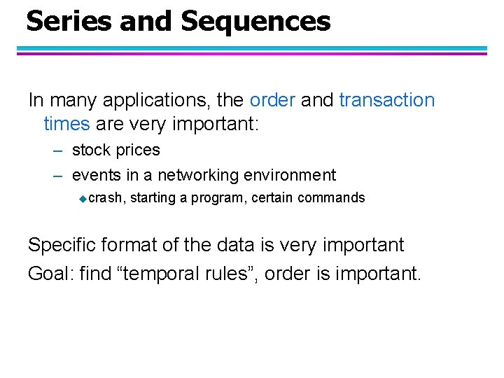
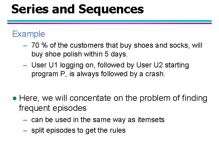
Series and Sequences In many applications, the order and transaction times are very important: – stock prices – events in a networking environment ucrash, starting a program, certain commands Specific format of the data is very important Goal: find “temporal rules”, order is important.

Series and Sequences Example – 70 % of the customers that buy shoes and socks, will buy shoe polish within 5 days. – User U 1 logging on, followed by User U 2 starting program P, is always followed by a crash. l Here, we will concentate on the problem of finding frequent episodes – can be used in the same way as itemsets – split episodes to get the rules

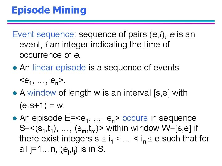
Episode Mining Event sequence: sequence of pairs (e, t), e is an event, t an integer indicating the time of occurrence of e. l An linear episode is a sequence of events <e 1, …, en>. l A window of length w is an interval [s, e] with (e-s+1) = w. l An episode E=<e 1, …, en> occurs in sequence S=<(s 1, t 1), …, (sm, tm)> within window W=[s, e] if there exist integers s i 1 < … < in e such that for all j=1…n, (ej, ij) is in S.

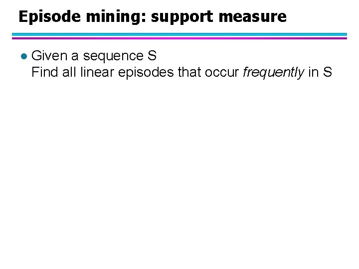
Episode mining: support measure l Given a sequence S Find all linear episodes that occur frequently in S

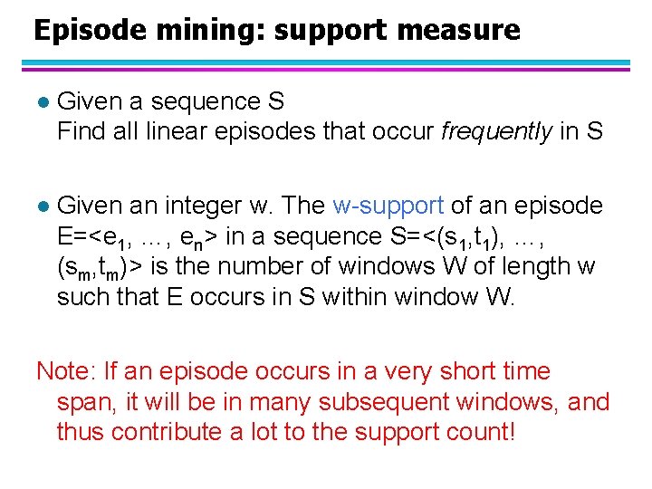
Episode mining: support measure l Given a sequence S Find all linear episodes that occur frequently in S l Given an integer w. The w-support of an episode E=<e 1, …, en> in a sequence S=<(s 1, t 1), …, (sm, tm)> is the number of windows W of length w such that E occurs in S within window W. Note: If an episode occurs in a very short time span, it will be in many subsequent windows, and thus contribute a lot to the support count!

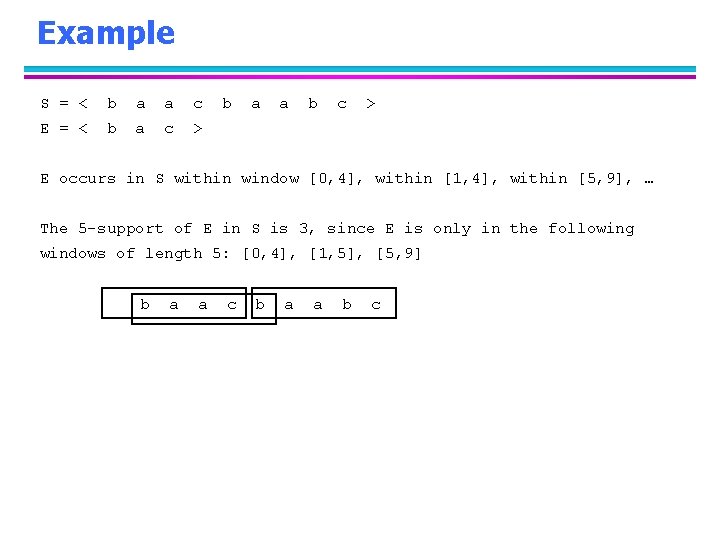
Example S = < b a a c E = < b a c > b a a b c > E occurs in S within window [0, 4], within [1, 4], within [5, 9], … The 5 -support of E in S is 3, since E is only in the following windows of length 5: [0, 4], [1, 5], [5, 9] b a a c b a a b c

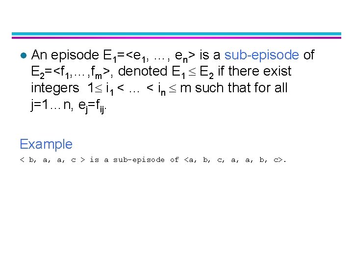
l An episode E 1=<e 1, …, en> is a sub-episode of E 2=<f 1, …, fm>, denoted E 1 E 2 if there exist integers 1 i 1 < … < in m such that for all j=1…n, ej=fij. Example < b, a, a, c > is a sub-episode of <a, b, c, a, a, b, c>.

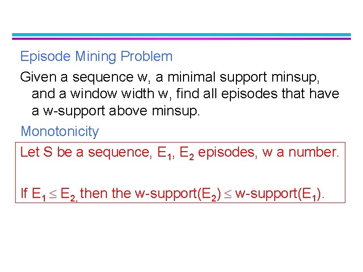
Episode Mining Problem Given a sequence w, a minimal support minsup, and a window width w, find all episodes that have a w-support above minsup. Monotonicity Let S be a sequence, E 1, E 2 episodes, w a number. If E 1 E 2, then the w-support(E 2) w-support(E 1).

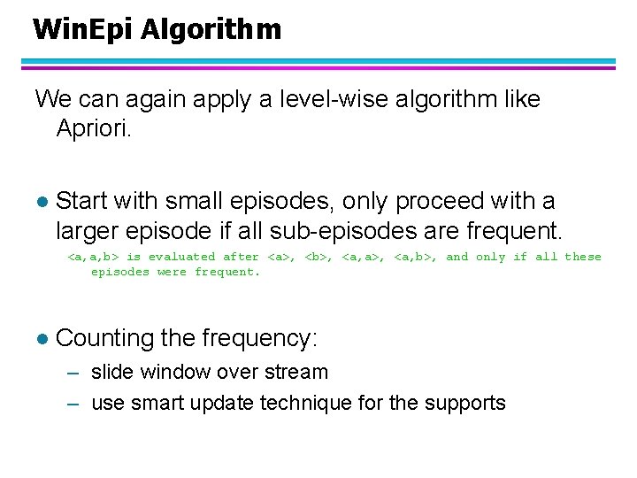
Win. Epi Algorithm We can again apply a level-wise algorithm like Apriori. l Start with small episodes, only proceed with a larger episode if all sub-episodes are frequent. <a, a, b> is evaluated after <a>, <b>, <a, a>, <a, b>, and only if all these episodes were frequent. l Counting the frequency: – slide window over stream – use smart update technique for the supports

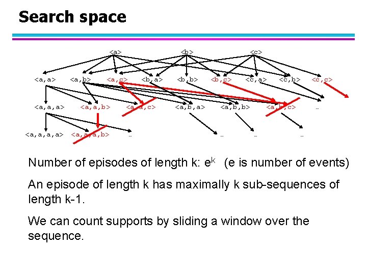
Search space <a> <a, b> <a, c> <a, a, a> <a, a, b> <a, a, a, a> <a, a, a, b> <b, a> <a, a, c> … <b, b> <a, b, a> <c> <b, c> <c, a> <a, b, b> … <c, b> <c, c> <a, b, c> … … … Number of episodes of length k: ek (e is number of events) An episode of length k has maximally k sub-sequences of length k-1. We can count supports by sliding a window over the sequence.

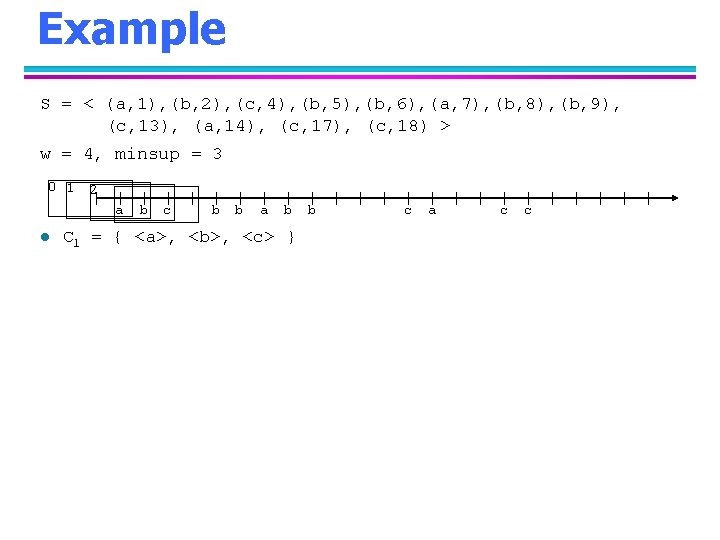
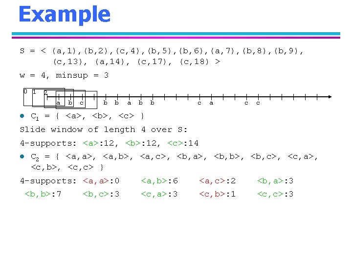
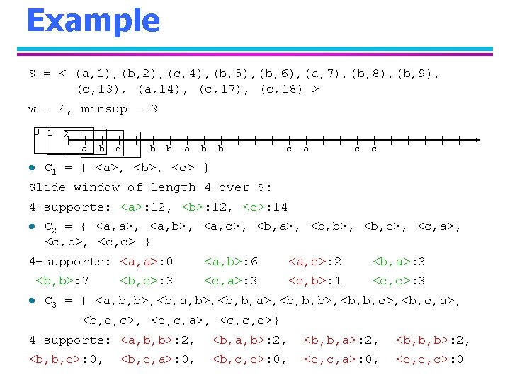
Example S = < (a, 1), (b, 2), (c, 4), (b, 5), (b, 6), (a, 7), (b, 8), (b, 9), (c, 13), (a, 14), (c, 17), (c, 18) > w = 4, minsup = 3 0 1 2 a l b c b b a b C 1 = { <a>, <b>, <c> } b c a c c

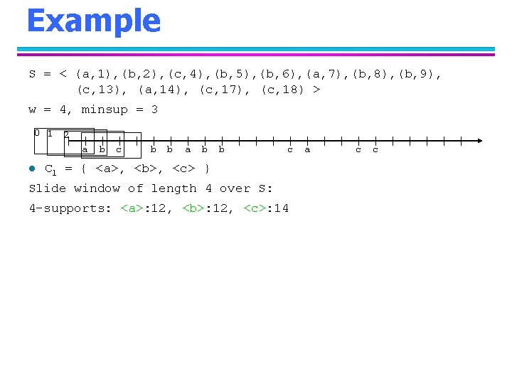
Example S = < (a, 1), (b, 2), (c, 4), (b, 5), (b, 6), (a, 7), (b, 8), (b, 9), (c, 13), (a, 14), (c, 17), (c, 18) > w = 4, minsup = 3 0 1 2 a l b c b b a b b c C 1 = { <a>, <b>, <c> } Slide window of length 4 over S: 4 -supports: <a>: 12, <b>: 12, <c>: 14 a c c

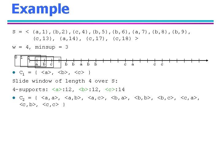
Example S = < (a, 1), (b, 2), (c, 4), (b, 5), (b, 6), (a, 7), (b, 8), (b, 9), (c, 13), (a, 14), (c, 17), (c, 18) > w = 4, minsup = 3 0 1 2 a l b c b b a b b c a c c C 1 = { <a>, <b>, <c> } Slide window of length 4 over S: 4 -supports: <a>: 12, <b>: 12, <c>: 14 l C 2 = { <a, a>, <a, b>, <a, c>, <b, a>, <b, b>, <b, c>, <c, a>, <c, b>, <c, c> }

Example S = < (a, 1), (b, 2), (c, 4), (b, 5), (b, 6), (a, 7), (b, 8), (b, 9), (c, 13), (a, 14), (c, 17), (c, 18) > w = 4, minsup = 3 0 1 2 a l b c b b a b b c a c c C 1 = { <a>, <b>, <c> } Slide window of length 4 over S: 4 -supports: <a>: 12, <b>: 12, <c>: 14 l C 2 = { <a, a>, <a, b>, <a, c>, <b, a>, <b, b>, <b, c>, <c, a>, <c, b>, <c, c> } 4 -supports: <a, a>: 0 <b, b>: 7 <b, c>: 3 <a, b>: 6 <a, c>: 2 <b, a>: 3 <c, b>: 1 <c, c>: 3

Example S = < (a, 1), (b, 2), (c, 4), (b, 5), (b, 6), (a, 7), (b, 8), (b, 9), (c, 13), (a, 14), (c, 17), (c, 18) > w = 4, minsup = 3 0 1 2 a l b c b b a b b c a c c C 1 = { <a>, <b>, <c> } Slide window of length 4 over S: 4 -supports: <a>: 12, <b>: 12, <c>: 14 l C 2 = { <a, a>, <a, b>, <a, c>, <b, a>, <b, b>, <b, c>, <c, a>, <c, b>, <c, c> } 4 -supports: <a, a>: 0 <b, b>: 7 l <b, c>: 3 <a, b>: 6 <a, c>: 2 <b, a>: 3 <c, b>: 1 <c, c>: 3 C 3 = { <a, b, b>, <b, a, b>, <b, b, a>, <b, b, b>, <b, b, c>, <b, c, a>, <b, c, c>, <c, c, a>, <c, c, c>} 4 -supports: <a, b, b>: 2, <b, a, b>: 2, <b, b, a>: 2, <b, b, b>: 2, <b, b, c>: 0, <b, c, c>: 0, <c, c, a>: 0, <c, c, c>: 0 <b, c, a>: 0,

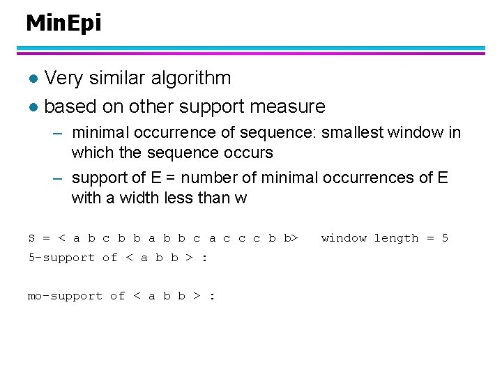
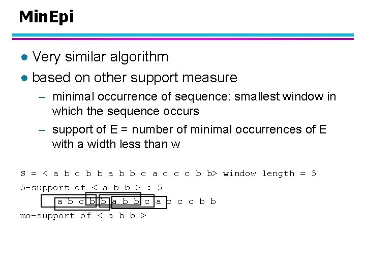
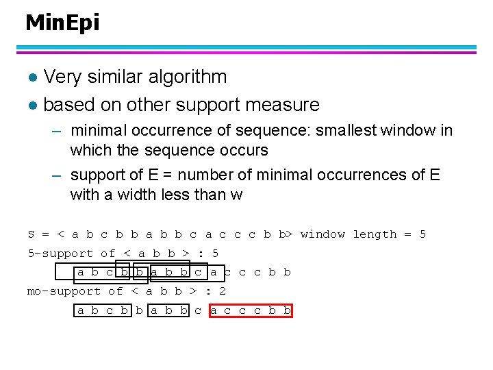
Min. Epi Very similar algorithm l based on other support measure l – minimal occurrence of sequence: smallest window in which the sequence occurs – support of E = number of minimal occurrences of E with a width less than w S = < a b c b b a b b c a c c c b b> 5 -support of < a b b > : mo-support of < a b b > : window length = 5

Min. Epi Very similar algorithm l based on other support measure l – minimal occurrence of sequence: smallest window in which the sequence occurs – support of E = number of minimal occurrences of E with a width less than w S = < a b c b b a b b c a c c c b b> window length = 5 5 -support of < a b b > : 5 a b c b b a b b c a c c c b b mo-support of < a b b >

Min. Epi Very similar algorithm l based on other support measure l – minimal occurrence of sequence: smallest window in which the sequence occurs – support of E = number of minimal occurrences of E with a width less than w S = < a b c b b a b b c a c c c b b> window length = 5 5 -support of < a b b > : 5 a b c b b a b b c a c c c b b mo-support of < a b b > : 2 a b c b b a b b c a c c c b b

Sequential Pattern Mining: Summary Mining sequential episodes l Two definitions of support: l – w-support – mo-support l Two algorithms: – Win. Epi – Min. Epi l Based on monotonicity principle – generate candidates levelwise – only count candidates without infrequent subsequences

Outline l Association Rule Mining – Frequent itemsets and association rules – Algorithms: Apriori and Eclat l Sequential Pattern Mining – Mining frequent episodes – Algorithms: Win. Epi and Min. Epi l Other types of patterns – strings, graphs, … – process mining

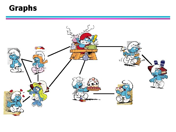
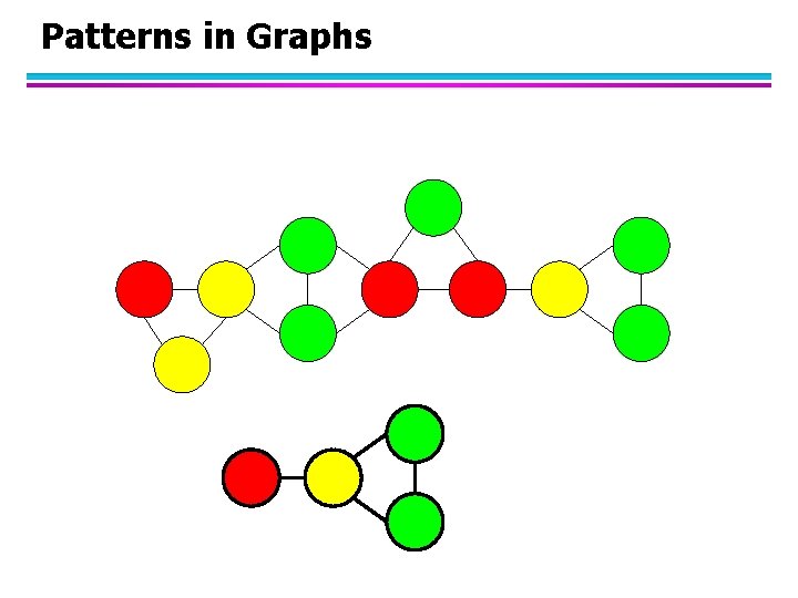
Other types of patterns l Sequence problems – Strings – Other types of sequences – Oher patterns in sequences l Graphs – Molecules – WWW – Social Networks l …

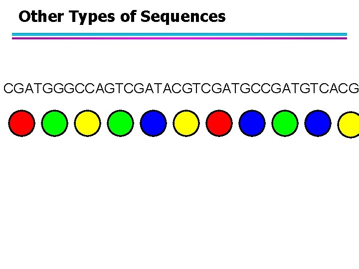
Other Types of Sequences CGATGGGCCAGTCGATACGTCGATGCCGATGTCACG

Other Patterns in Sequences l l Substrings Regular expressions (bb|[^b]{2}) Partial orders Directed Acyclic Graphs

Graphs

Patterns in Graphs

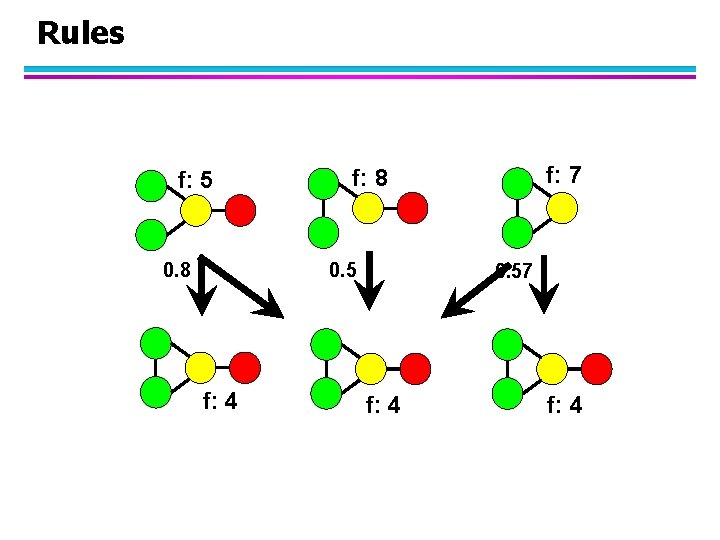
Rules f: 5 0. 8 f: 4 f: 7 f: 8 0. 57 f: 4

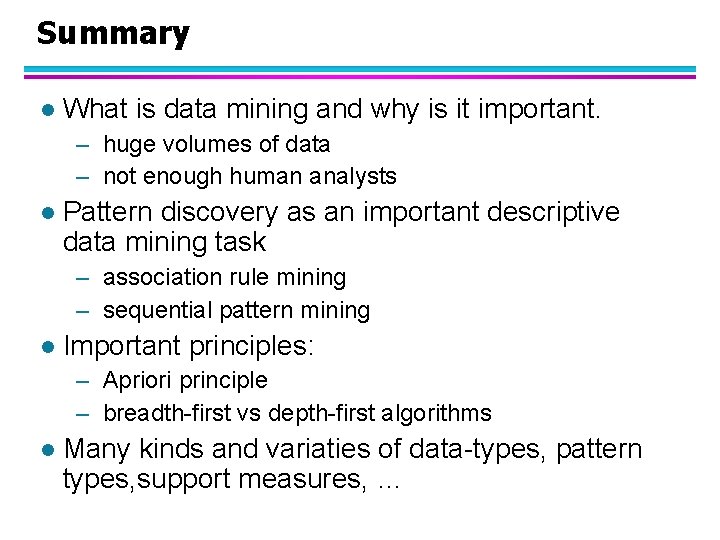
Summary l What is data mining and why is it important. – huge volumes of data – not enough human analysts l Pattern discovery as an important descriptive data mining task – association rule mining – sequential pattern mining l Important principles: – Apriori principle – breadth-first vs depth-first algorithms l Many kinds and variaties of data-types, pattern types, support measures, …