Data Mining Association Rule Mining 2262021 Data Mining

Data Mining Association Rule Mining 2/26/2021 Data Mining 1

Mining Association Rules in Large Databases n Association rule mining n Algorithms for scalable mining of (single-dimensional Boolean) association rules in transactional databases n Mining various kinds of association/correlation rules n Applications/extensions of frequent pattern mining n Summary 2/26/2021 Data Mining 2

What Is Association Mining? n n Association rule mining: n Finding frequent patterns, associations, correlations, or causal structures among sets of items or objects in transaction databases, relational databases, and other information repositories. n Frequent pattern: pattern (set of items, sequence, etc. ) that occurs frequently in a database Motivation: finding regularities in data n What products were often purchased together? — Beer and diapers? ! n What are the subsequent purchases after buying a PC? n What kinds of DNA are sensitive to this new drug? n Can we automatically classify web documents? 2/26/2021 Data Mining 3

Why Is Frequent Pattern or Association Mining an Essential Task in Data Mining? n Foundation for many essential data mining tasks n n Association, correlation, causality Sequential patterns, temporal or cyclic association, partial periodicity, spatial and multimedia association Associative classification, cluster analysis, iceberg cube Broad applications n Basket data analysis, cross-marketing, catalog design, sale campaign analysis n Web log (click stream) analysis, DNA sequence analysis, etc. 2/26/2021 Data Mining 4

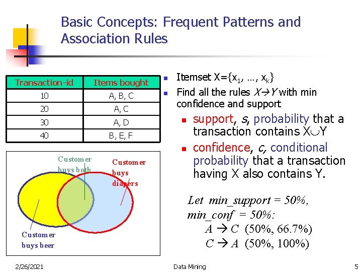
Basic Concepts: Frequent Patterns and Association Rules Transaction-id Items bought n 10 A, B, C n 20 A, C 30 A, D 40 B, E, F Itemset X={x 1, …, xk} Find all the rules X Y with min confidence and support n n Customer buys both Customer buys beer 2/26/2021 Customer buys diapers support, s, probability that a transaction contains X Y confidence, c, conditional probability that a transaction having X also contains Y. Let min_support = 50%, min_conf = 50%: A C (50%, 66. 7%) C A (50%, 100%) Data Mining 5

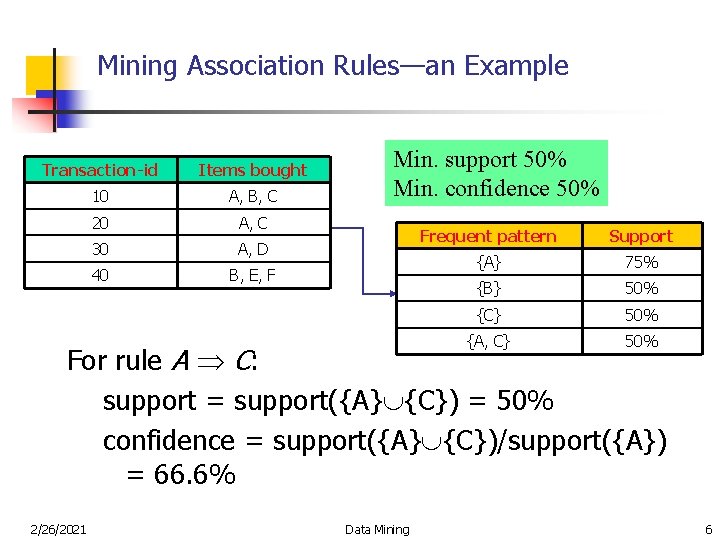
Mining Association Rules—an Example Transaction-id Items bought 10 A, B, C 20 A, C 30 A, D 40 B, E, F Min. support 50% Min. confidence 50% Frequent pattern Support {A} 75% {B} 50% {C} 50% {A, C} 50% For rule A C: support = support({A} {C}) = 50% confidence = support({A} {C})/support({A}) = 66. 6% 2/26/2021 Data Mining 6

Chapter 6: Mining Association Rules in Large Databases n Association rule mining n Algorithms for scalable mining of (single-dimensional Boolean) association rules in transactional databases n Mining various kinds of association/correlation rules n Applications/extensions of frequent pattern mining n Summary 2/26/2021 Data Mining 7

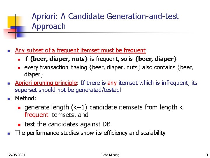
Apriori: A Candidate Generation-and-test Approach n n n Any subset of a frequent itemset must be frequent n if {beer, diaper, nuts} is frequent, so is {beer, diaper} n every transaction having {beer, diaper, nuts} also contains {beer, diaper} Apriori pruning principle: If there is any itemset which is infrequent, its superset should not be generated/tested! Method: n n n generate length (k+1) candidate itemsets from length k frequent itemsets, and test the candidates against DB The performance studies show its efficiency and scalability 2/26/2021 Data Mining 8

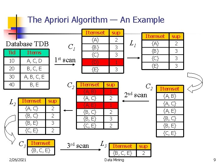
The Apriori Algorithm — An Example Database TDB Tid Items 10 A, C, D 20 B, C, E 30 A, B, C, E 40 B, E L 2 {A} 2 {B} 3 {C} 3 {D} 1 {E} 3 1 st scan C 2 sup {A, C} 2 {B, E} 3 {C, E} 2 2/26/2021 sup C 1 Itemset C 3 Itemset {B, C, E} Itemset {A, B} {A, C} {A, E} {B, C} {B, E} {C, E} sup 1 2 3 2 L 1 Itemset sup {A} 2 {B} 3 {C} 3 {E} 3 C 2 2 nd scan Itemset {A, B} {A, C} {A, E} {B, C} {B, E} {C, E} 3 rd scan L 3 Itemset {B, C, E} Data Mining sup 2 9

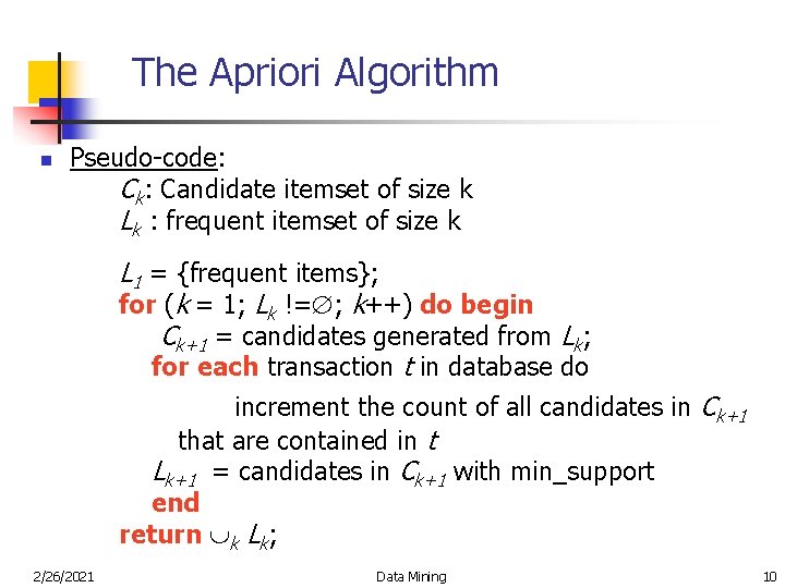
The Apriori Algorithm n Pseudo-code: Ck: Candidate itemset of size k Lk : frequent itemset of size k L 1 = {frequent items}; for (k = 1; Lk != ; k++) do begin Ck+1 = candidates generated from Lk; for each transaction t in database do increment the count of all candidates in Ck+1 that are contained in t Lk+1 = candidates in Ck+1 with min_support end return k Lk; 2/26/2021 Data Mining 10

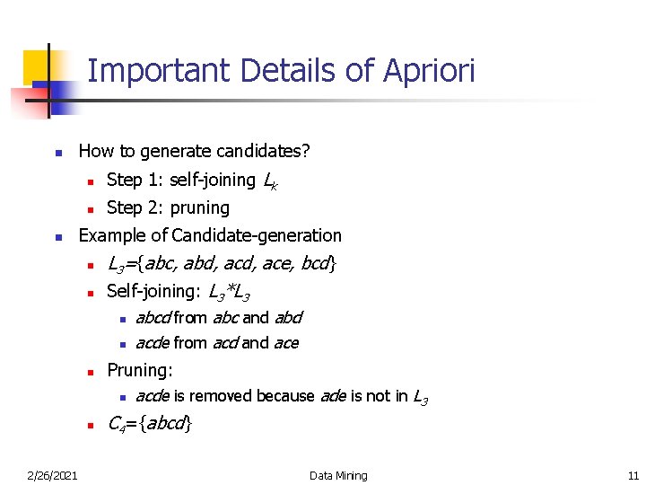
Important Details of Apriori n n How to generate candidates? n Step 1: self-joining Lk n Step 2: pruning Example of Candidate-generation n n L 3={abc, abd, ace, bcd} Self-joining: L 3*L 3 n n 2/26/2021 abcd from abc and abd acde from acd and ace Pruning: n acde is removed because ade is not in L 3 C 4={abcd} Data Mining 11

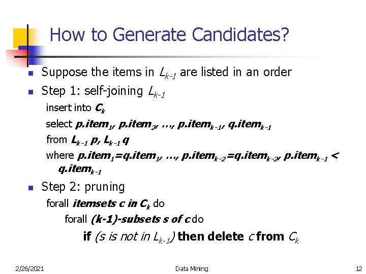
How to Generate Candidates? n Suppose the items in Lk-1 are listed in an order n Step 1: self-joining Lk-1 insert into Ck select p. item 1, p. item 2, …, p. itemk-1, q. itemk-1 from Lk-1 p, Lk-1 q where p. item 1=q. item 1, …, p. itemk-2=q. itemk-2, p. itemk-1 < q. itemk-1 n Step 2: pruning forall itemsets c in Ck do forall (k-1)-subsets s of c do if (s is not in Lk-1) then delete c from Ck 2/26/2021 Data Mining 12

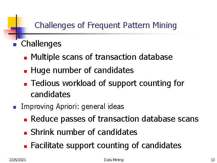
Challenges of Frequent Pattern Mining n Challenges n Multiple scans of transaction database n Huge number of candidates n n Tedious workload of support counting for candidates Improving Apriori: general ideas n Reduce passes of transaction database scans n Shrink number of candidates n Facilitate support counting of candidates 2/26/2021 Data Mining 13

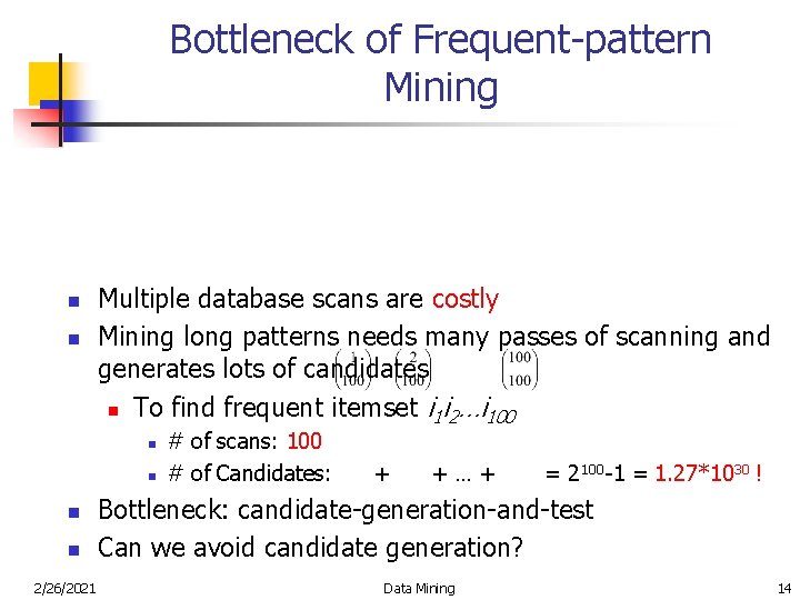
Bottleneck of Frequent-pattern Mining n n Multiple database scans are costly Mining long patterns needs many passes of scanning and generates lots of candidates n To find frequent itemset i 1 i 2…i 100 n n 2/26/2021 # of scans: 100 # of Candidates: + +…+ = 2100 -1 = 1. 27*1030 ! Bottleneck: candidate-generation-and-test Can we avoid candidate generation? Data Mining 14

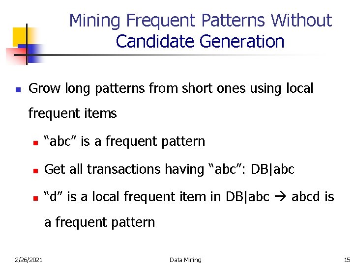
Mining Frequent Patterns Without Candidate Generation n Grow long patterns from short ones using local frequent items n “abc” is a frequent pattern n Get all transactions having “abc”: DB|abc n “d” is a local frequent item in DB|abc abcd is a frequent pattern 2/26/2021 Data Mining 15

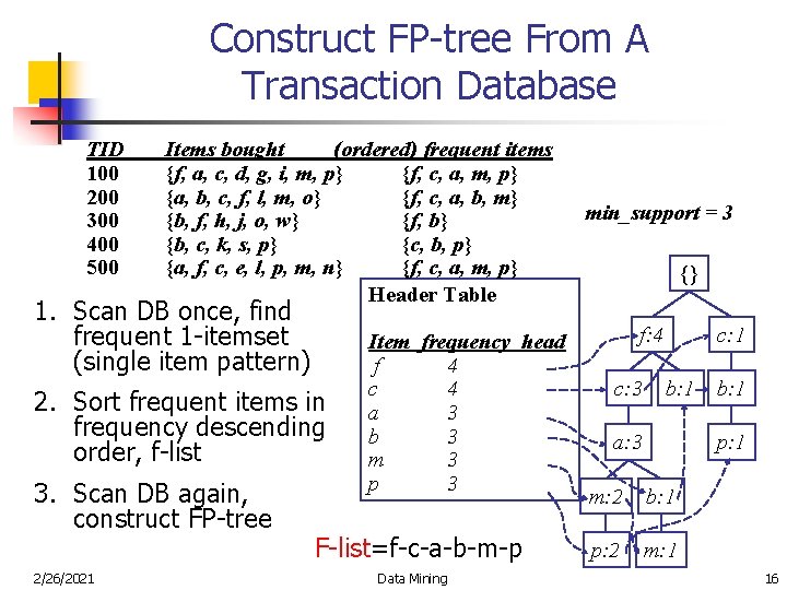
Construct FP-tree From A Transaction Database TID 100 200 300 400 500 Items bought (ordered) frequent items {f, a, c, d, g, i, m, p} {f, c, a, m, p} {a, b, c, f, l, m, o} {f, c, a, b, m} {b, f, h, j, o, w} {f, b} {b, c, k, s, p} {c, b, p} {a, f, c, e, l, p, m, n} {f, c, a, m, p} Header Table 1. Scan DB once, find frequent 1 -itemset (single item pattern) 2. Sort frequent items in frequency descending order, f-list 3. Scan DB again, construct FP-tree 2/26/2021 Item frequency head f 4 c 4 a 3 b 3 m 3 p 3 F-list=f-c-a-b-m-p Data Mining min_support = 3 {} f: 4 c: 3 c: 1 b: 1 a: 3 b: 1 p: 1 m: 2 b: 1 p: 2 m: 1 16

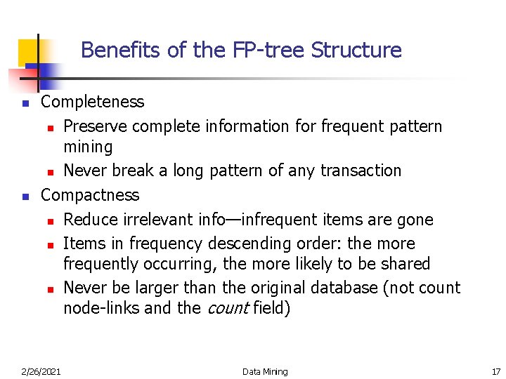
Benefits of the FP-tree Structure n n Completeness n Preserve complete information for frequent pattern mining n Never break a long pattern of any transaction Compactness n Reduce irrelevant info—infrequent items are gone n Items in frequency descending order: the more frequently occurring, the more likely to be shared n Never be larger than the original database (not count node-links and the count field) 2/26/2021 Data Mining 17

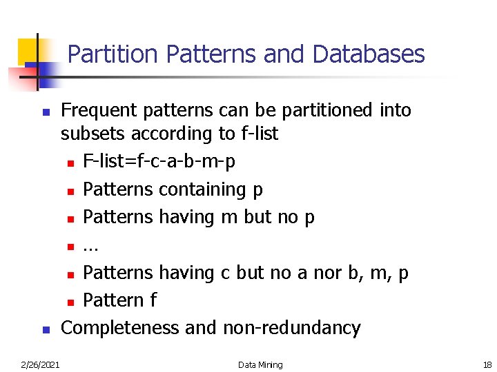
Partition Patterns and Databases n n 2/26/2021 Frequent patterns can be partitioned into subsets according to f-list n F-list=f-c-a-b-m-p n Patterns containing p n Patterns having m but no p n … n Patterns having c but no a nor b, m, p n Pattern f Completeness and non-redundancy Data Mining 18

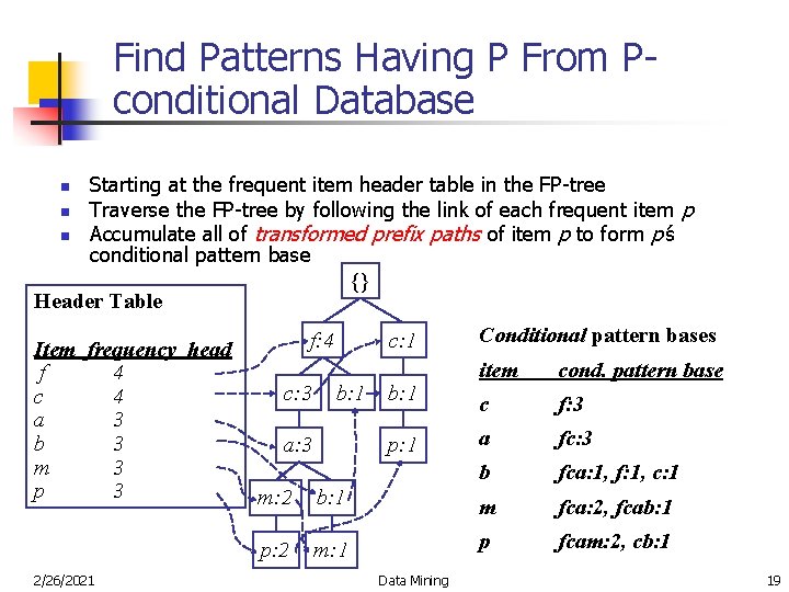
Find Patterns Having P From Pconditional Database n n n Starting at the frequent item header table in the FP-tree Traverse the FP-tree by following the link of each frequent item p Accumulate all of transformed prefix paths of item p to form p’s conditional pattern base {} Header Table Item frequency head f 4 c 4 a 3 b 3 m 3 p 3 2/26/2021 f: 4 c: 3 c: 1 b: 1 a: 3 b: 1 p: 1 Conditional pattern bases item cond. pattern base c f: 3 a fc: 3 b fca: 1, f: 1, c: 1 m: 2 b: 1 m fca: 2, fcab: 1 p: 2 m: 1 p fcam: 2, cb: 1 Data Mining 19

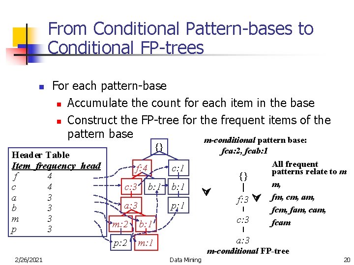
From Conditional Pattern-bases to Conditional FP-trees n For each pattern-base n Accumulate the count for each item in the base n Construct the FP-tree for the frequent items of the pattern base m-conditional pattern base: Header Table Item frequency head f 4 c 4 a 3 b 3 m 3 p 3 2/26/2021 {} f: 4 c: 3 fca: 2, fcab: 1 c: 1 b: 1 a: 3 b: 1 {} p: 1 f: 3 m: 2 b: 1 c: 3 p: 2 m: 1 a: 3 All frequent patterns relate to m m, fm, cm, am, fcm, fam, cam, fcam m-conditional FP-tree Data Mining 20

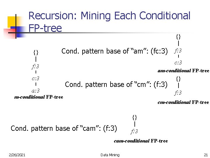
Recursion: Mining Each Conditional FP-tree {} {} Cond. pattern base of “am”: (fc: 3) c: 3 f: 3 c: 3 a: 3 f: 3 am-conditional FP-tree Cond. pattern base of “cm”: (f: 3) {} f: 3 m-conditional FP-tree cm-conditional FP-tree {} Cond. pattern base of “cam”: (f: 3) f: 3 cam-conditional FP-tree 2/26/2021 Data Mining 21

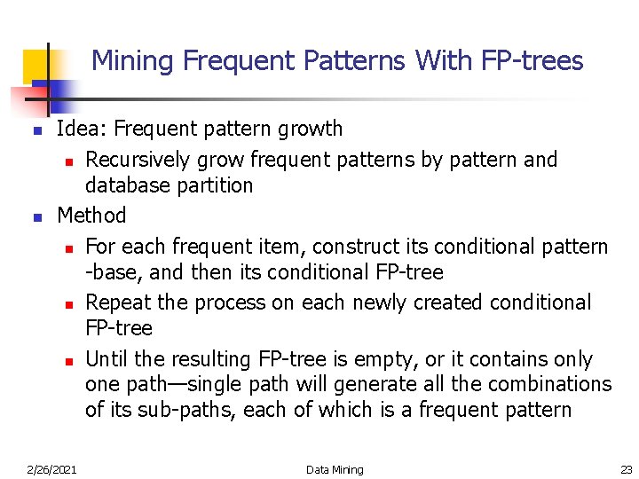
Mining Frequent Patterns With FP-trees n n Idea: Frequent pattern growth n Recursively grow frequent patterns by pattern and database partition Method n For each frequent item, construct its conditional pattern -base, and then its conditional FP-tree n Repeat the process on each newly created conditional FP-tree n Until the resulting FP-tree is empty, or it contains only one path—single path will generate all the combinations of its sub-paths, each of which is a frequent pattern 2/26/2021 Data Mining 23

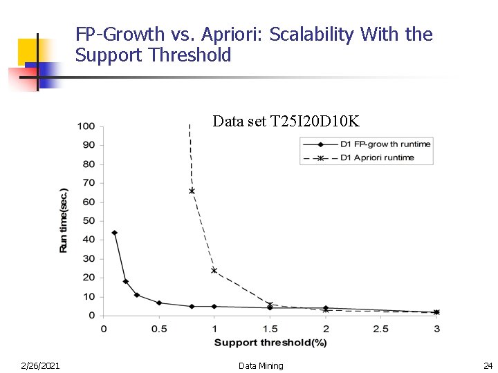
FP-Growth vs. Apriori: Scalability With the Support Threshold Data set T 25 I 20 D 10 K 2/26/2021 Data Mining 24

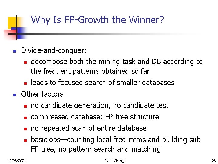
Why Is FP-Growth the Winner? n Divide-and-conquer: n n n decompose both the mining task and DB according to the frequent patterns obtained so far leads to focused search of smaller databases Other factors n no candidate generation, no candidate test n compressed database: FP-tree structure n no repeated scan of entire database n 2/26/2021 basic ops—counting local freq items and building sub FP-tree, no pattern search and matching Data Mining 26

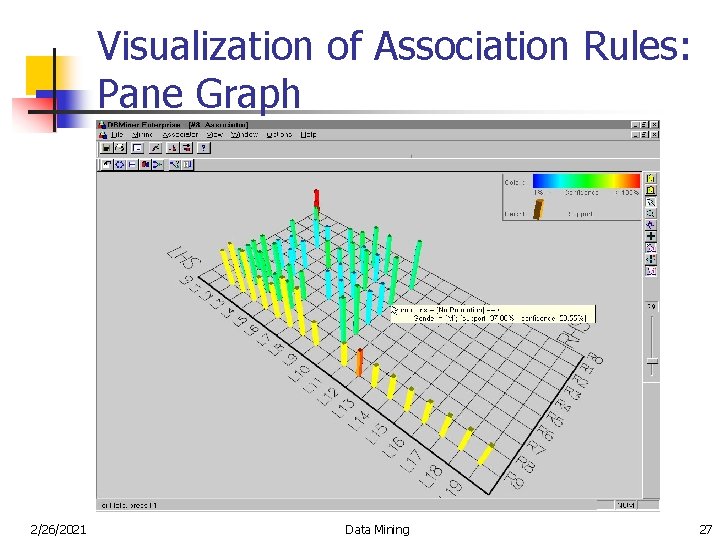
Visualization of Association Rules: Pane Graph 2/26/2021 Data Mining 27

Other Algorithms for Association Rules Mining n n n 2/26/2021 Partition Algorithm Sampling Method Dynamic Itemset Counting Data Mining 29

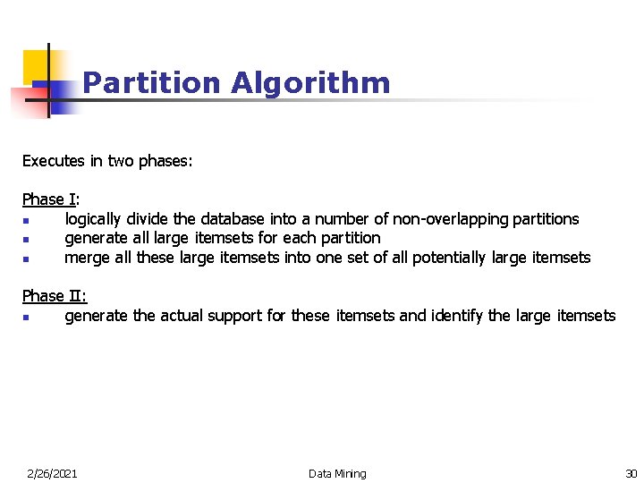
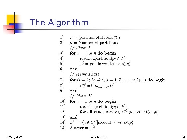
Partition Algorithm Executes in two phases: Phase I: n logically divide the database into a number of non-overlapping partitions n generate all large itemsets for each partition n merge all these large itemsets into one set of all potentially large itemsets Phase II: n generate the actual support for these itemsets and identify the large itemsets 2/26/2021 Data Mining 30

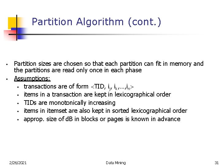
Partition Algorithm (cont. ) w w Partition sizes are chosen so that each partition can fit in memory and the partitions are read only once in each phase Assumptions: w transactions are of form TID, ij, ik, …, in w items in a transaction are kept in lexicographical order w TIDs are monotonically increasing w items in itemset are also kept in sorted lexicographical order w approp. size of d. B in blocks or pages is known in advance 2/26/2021 Data Mining 31

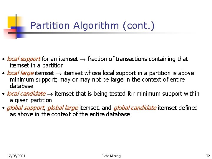
Partition Algorithm (cont. ) • local support for an itemset fraction of transactions containing that itemset in a partition • local large itemset whose local support in a partition is above minimum support; may or may not be large in the context of entire database • local candidate itemset that is being tested for minimum support within a given partition • global support, global large itemset, and global candidate itemset defined as above in the context of the entire database 2/26/2021 Data Mining 32

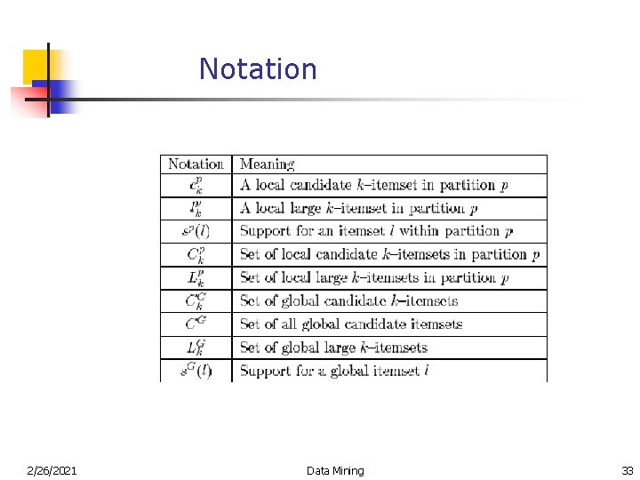
Notation 2/26/2021 Data Mining 33

The Algorithm 2/26/2021 Data Mining 34

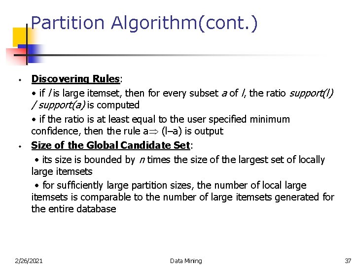
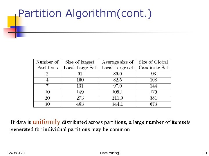
Partition Algorithm(cont. ) w w Discovering Rules: • if l is large itemset, then for every subset a of l, the ratio support(l) / support(a) is computed • if the ratio is at least equal to the user specified minimum confidence, then the rule a (l–a) is output Size of the Global Candidate Set: • its size is bounded by n times the size of the largest set of locally large itemsets • for sufficiently large partition sizes, the number of local large itemsets is comparable to the number of large itemsets generated for the entire database 2/26/2021 Data Mining 37

Partition Algorithm(cont. ) If data is uniformly distributed across partitions, a large number of itemsets generated for individual partitions may be common 2/26/2021 Data Mining 38

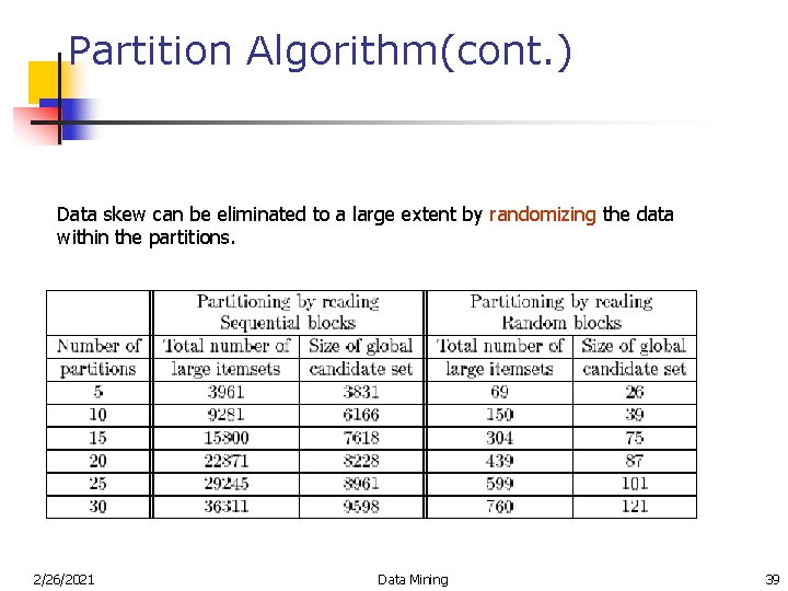
Partition Algorithm(cont. ) Data skew can be eliminated to a large extent by randomizing the data within the partitions. 2/26/2021 Data Mining 39

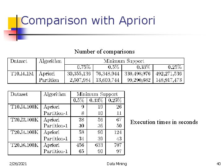
Comparison with Apriori Number of comparisons Execution times in seconds 2/26/2021 Data Mining 40

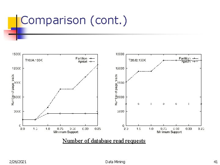
Comparison (cont. ) Number of database read requests 2/26/2021 Data Mining 41

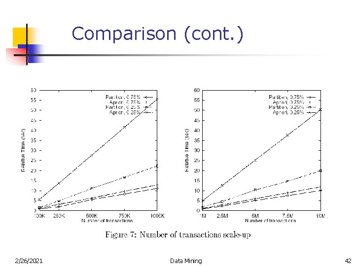
Comparison (cont. ) 2/26/2021 Data Mining 42

Partition Algorithm Highlights: w Achieved both CPU and I/O improvements over Apriori w Scans the database twice w Scales linearly with number of transactions w Inherent parallelism in the algorithm can be exploited for the implementation on a parallel machine 2/26/2021 Data Mining 44

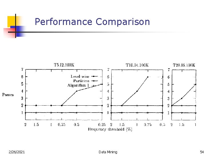
Sampling Algorithm § § § Makes one full pass, two passes in the worst case Pick a random sample, find all association rules and then verify the results In very rare cases not all the association rules are produced in the first scan because the algorithm is probabilistic Samples small enough to be handled totally in main memory give reasonably accurate results Tradeoff accuracy against efficiency 2/26/2021 Data Mining 45

Sampling Step • • A superset can be determined efficiently by applying the level-wise method on the sample in main memory, and by using a lowered frequency threshold In terms of partition algorithm, discover locally frequent sets from one part only, and with a lower threshold 2/26/2021 Data Mining 46

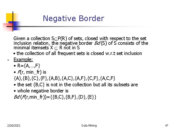
Negative Border w Given a collection S P(R) of sets, closed with respect to the set inclusion relation, the negative border Bd-(S) of S consists of the minimal itemsets X R not in S • the collection of all frequent sets is closed w. r. t set inclusion Example: • R={A, …, F} • F(r, min_fr) is {A}, {B}, {C}, {F}, {A, B}, {A, C}, {A, F}, {C, F}, {A, C, F} • the set {B, C} is not in the collection but all its subsets are • whole negative border is Bd-(F(r, min_fr))={{B, C}, {B, F}, {D}, {E}} 2/26/2021 Data Mining 47

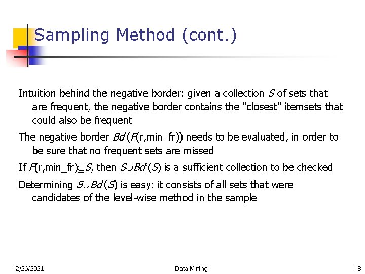
Sampling Method (cont. ) Intuition behind the negative border: given a collection S of sets that are frequent, the negative border contains the “closest” itemsets that could also be frequent The negative border Bd-(F(r, min_fr)) needs to be evaluated, in order to be sure that no frequent sets are missed If F(r, min_fr) S, then S Bd-(S) is a sufficient collection to be checked Determining S Bd-(S) is easy: it consists of all sets that were candidates of the level-wise method in the sample 2/26/2021 Data Mining 48

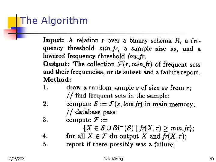
The Algorithm 2/26/2021 Data Mining 49

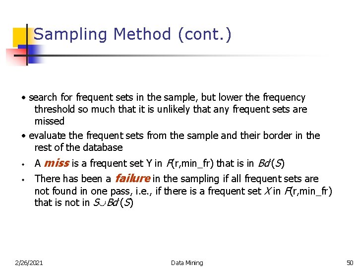
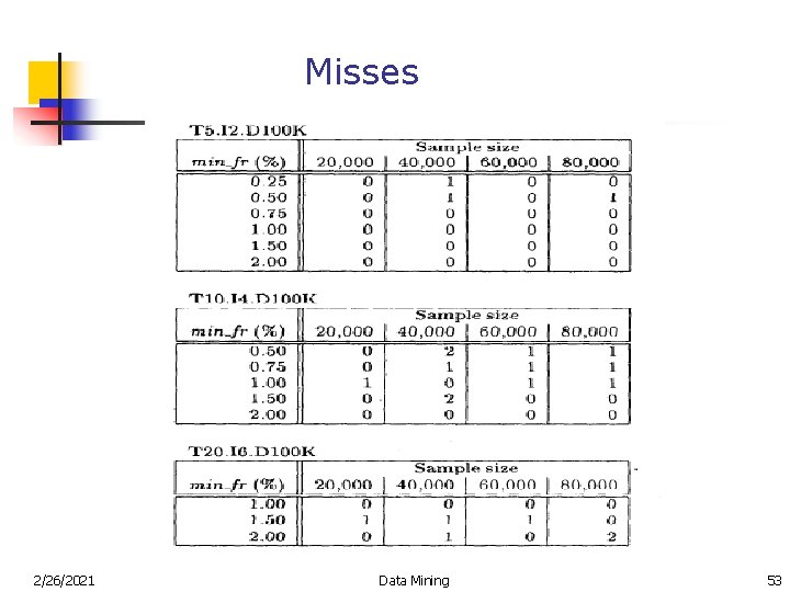
Sampling Method (cont. ) • search for frequent sets in the sample, but lower the frequency threshold so much that it is unlikely that any frequent sets are missed • evaluate the frequent sets from the sample and their border in the rest of the database w w A miss is a frequent set Y in F(r, min_fr) that is in Bd-(S) There has been a failure in the sampling if all frequent sets are not found in one pass, i. e. , if there is a frequent set X in F(r, min_fr) that is not in S Bd-(S) 2/26/2021 Data Mining 50

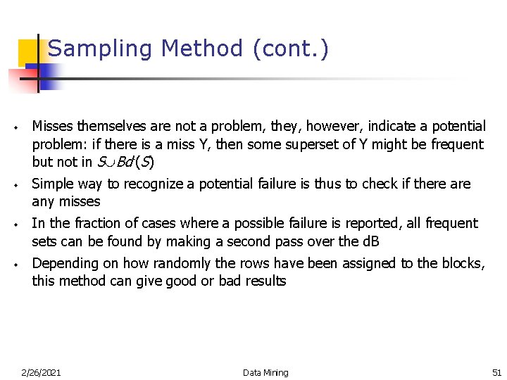
Sampling Method (cont. ) w w Misses themselves are not a problem, they, however, indicate a potential problem: if there is a miss Y, then some superset of Y might be frequent but not in S Bd-(S) Simple way to recognize a potential failure is thus to check if there any misses In the fraction of cases where a possible failure is reported, all frequent sets can be found by making a second pass over the d. B Depending on how randomly the rows have been assigned to the blocks, this method can give good or bad results 2/26/2021 Data Mining 51

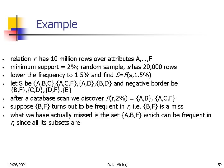
Example w w w w relation r has 10 million rows over attributes A, …, F minimum support = 2%; random sample, s has 20, 000 rows lower the frequency to 1. 5% and find S=F(s, 1. 5%) let S be {A, B, C}, {A, C, F}, {A, D}, {B, D} and negative border be {B, F}, {C, D}, {D, F}, {E} after a database scan we discover F(r, 2%) = {A, B}, {A, C, F} suppose {B, F} turns out to be frequent in r, i. e. {B, F} is a miss what we have actually missed is the set {A, B, F} which can be frequent in r, since all its subsets are 2/26/2021 Data Mining 52

Misses 2/26/2021 Data Mining 53

Performance Comparison 2/26/2021 Data Mining 54

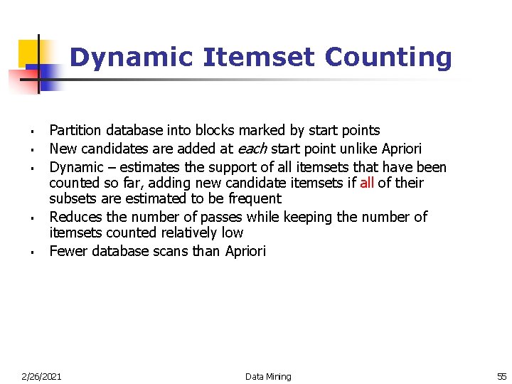
Dynamic Itemset Counting § § § Partition database into blocks marked by start points New candidates are added at each start point unlike Apriori Dynamic – estimates the support of all itemsets that have been counted so far, adding new candidate itemsets if all of their subsets are estimated to be frequent Reduces the number of passes while keeping the number of itemsets counted relatively low Fewer database scans than Apriori 2/26/2021 Data Mining 55

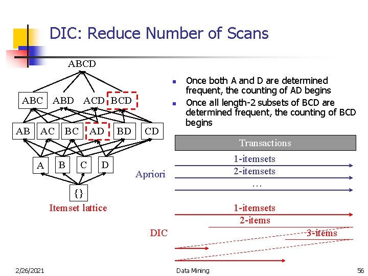
DIC: Reduce Number of Scans ABCD n ABC ABD ACD BCD AB AC BC AD BD n CD Once both A and D are determined frequent, the counting of AD begins Once all length-2 subsets of BCD are determined frequent, the counting of BCD begins Transactions A B C D 1 -itemsets 2 -itemsets … Apriori {} Itemset lattice 1 -itemsets 2 -items DIC 2/26/2021 3 -items Data Mining 56

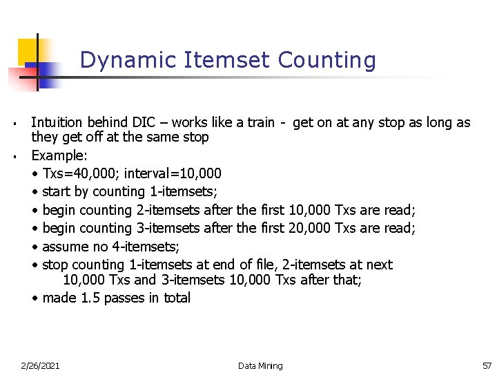
Dynamic Itemset Counting § § Intuition behind DIC – works like a train - get on at any stop as long as they get off at the same stop Example: • Txs=40, 000; interval=10, 000 • start by counting 1 -itemsets; • begin counting 2 -itemsets after the first 10, 000 Txs are read; • begin counting 3 -itemsets after the first 20, 000 Txs are read; • assume no 4 -itemsets; • stop counting 1 -itemsets at end of file, 2 -itemsets at next 10, 000 Txs and 3 -itemsets 10, 000 Txs after that; • made 1. 5 passes in total 2/26/2021 Data Mining 57

Mining Association Rules in Large Databases n Association rule mining n Algorithms for scalable mining of (single-dimensional Boolean) association rules in transactional databases n Mining various kinds of association/correlation rules n Applications/extensions of frequent pattern mining n Summary 2/26/2021 Data Mining 58

Mining Various Kinds of Rules or Regularities n Multi-level, quantitative association rules, correlation and causality, ratio rules, sequential patterns, emerging patterns, temporal associations, partial periodicity n Classification, clustering, iceberg cubes, etc. 2/26/2021 Data Mining 59

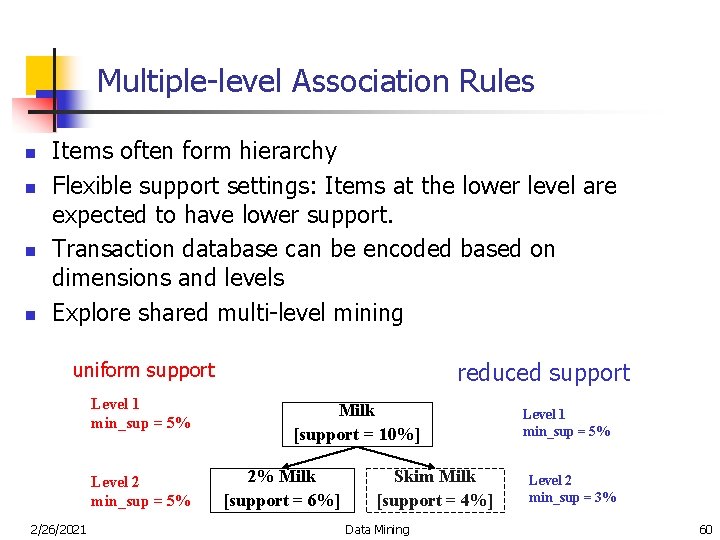
Multiple-level Association Rules n n Items often form hierarchy Flexible support settings: Items at the lower level are expected to have lower support. Transaction database can be encoded based on dimensions and levels Explore shared multi-level mining reduced support uniform support Level 1 min_sup = 5% Level 2 min_sup = 5% 2/26/2021 Milk [support = 10%] 2% Milk [support = 6%] Skim Milk [support = 4%] Data Mining Level 1 min_sup = 5% Level 2 min_sup = 3% 60

ML/MD Associations with Flexible Support Constraints n Why flexible support constraints? n Real life occurrence frequencies vary greatly n n n Diamond, watch, pen in a shopping basket Uniform support may not be an interesting model A flexible model n n n The lower-level, the more dimension combination, and the long pattern length, usually the smaller support General rules should be easy to specify and understand Special items and special group of items may be specified individually and have higher priority 2/26/2021 Data Mining 61

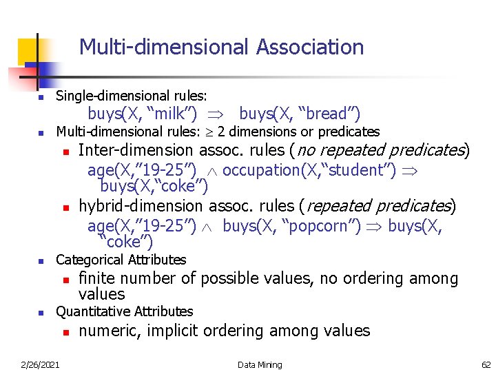
Multi-dimensional Association n Single-dimensional rules: buys(X, “milk”) buys(X, “bread”) n Multi-dimensional rules: 2 dimensions or predicates n n n Categorical Attributes n n Inter-dimension assoc. rules (no repeated predicates) age(X, ” 19 -25”) occupation(X, “student”) buys(X, “coke”) hybrid-dimension assoc. rules (repeated predicates) age(X, ” 19 -25”) buys(X, “popcorn”) buys(X, “coke”) finite number of possible values, no ordering among values Quantitative Attributes n 2/26/2021 numeric, implicit ordering among values Data Mining 62

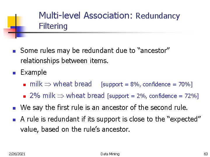
Multi-level Association: Redundancy Filtering n n Some rules may be redundant due to “ancestor” relationships between items. Example n milk wheat bread n 2% milk wheat bread [support = 2%, confidence = 72%] [support = 8%, confidence = 70%] We say the first rule is an ancestor of the second rule. A rule is redundant if its support is close to the “expected” value, based on the rule’s ancestor. 2/26/2021 Data Mining 63

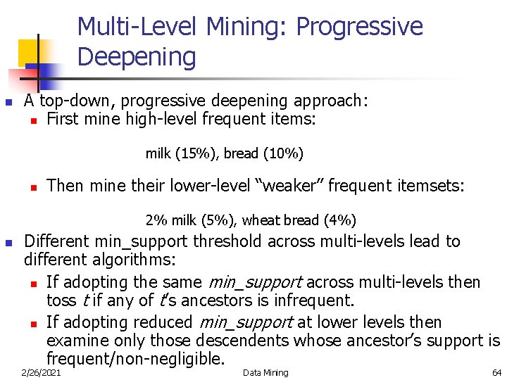
Multi-Level Mining: Progressive Deepening n A top-down, progressive deepening approach: n First mine high-level frequent items: milk (15%), bread (10%) n Then mine their lower-level “weaker” frequent itemsets: 2% milk (5%), wheat bread (4%) n Different min_support threshold across multi-levels lead to different algorithms: n If adopting the same min_support across multi-levels then toss t if any of t’s ancestors is infrequent. n If adopting reduced min_support at lower levels then examine only those descendents whose ancestor’s support is frequent/non-negligible. 2/26/2021 Data Mining 64

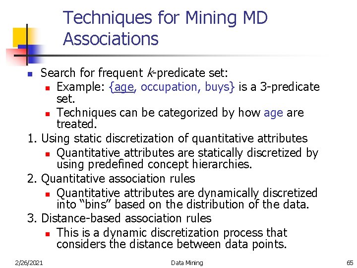
Techniques for Mining MD Associations Search for frequent k-predicate set: n Example: {age, occupation, buys} is a 3 -predicate set. n Techniques can be categorized by how age are treated. 1. Using static discretization of quantitative attributes n Quantitative attributes are statically discretized by using predefined concept hierarchies. 2. Quantitative association rules n Quantitative attributes are dynamically discretized into “bins” based on the distribution of the data. 3. Distance-based association rules n This is a dynamic discretization process that considers the distance between data points. n 2/26/2021 Data Mining 65

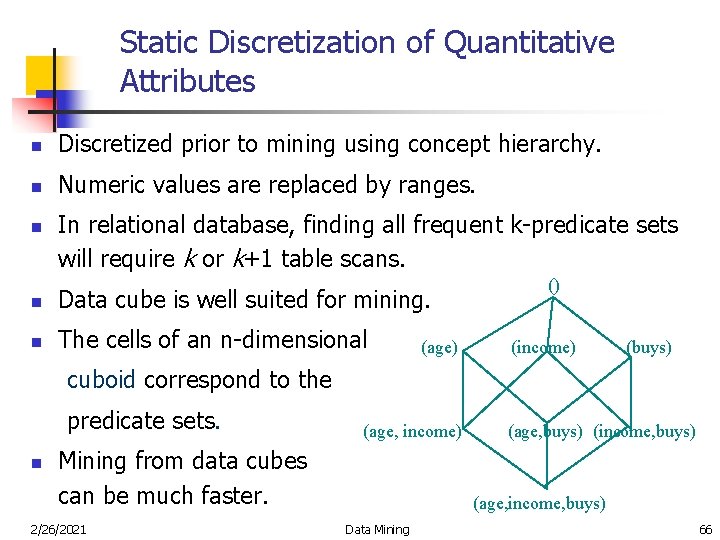
Static Discretization of Quantitative Attributes n Discretized prior to mining using concept hierarchy. n Numeric values are replaced by ranges. n In relational database, finding all frequent k-predicate sets will require k or k+1 table scans. n Data cube is well suited for mining. n The cells of an n-dimensional (age) () (income) (buys) cuboid correspond to the predicate sets. n (age, income) Mining from data cubes can be much faster. 2/26/2021 (age, buys) (income, buys) (age, income, buys) Data Mining 66

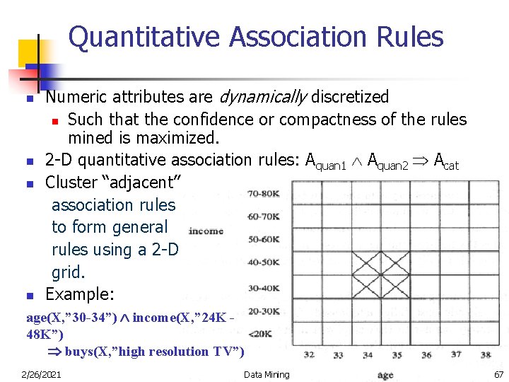
Quantitative Association Rules n n Numeric attributes are dynamically discretized n Such that the confidence or compactness of the rules mined is maximized. 2 -D quantitative association rules: Aquan 1 Aquan 2 Acat Cluster “adjacent” association rules to form general rules using a 2 -D grid. Example: age(X, ” 30 -34”) income(X, ” 24 K 48 K”) buys(X, ”high resolution TV”) 2/26/2021 Data Mining 67

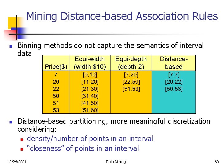
Mining Distance-based Association Rules n n Binning methods do not capture the semantics of interval data Distance-based partitioning, more meaningful discretization considering: n density/number of points in an interval n “closeness” of points in an interval 2/26/2021 Data Mining 68

Interestingness Measurements n Objective measures Two popular measurements: ¶ support; and · n 2/26/2021 confidence Subjective measures A rule (pattern) is interesting if ¶ it is unexpected (surprising to the user); and/or · actionable (the user can do something with it) Data Mining 69

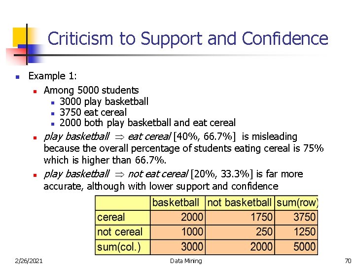
Criticism to Support and Confidence n Example 1: n Among 5000 students n 3000 play basketball n 3750 eat cereal n 2000 both play basketball and eat cereal n play basketball eat cereal [40%, 66. 7%] is misleading because the overall percentage of students eating cereal is 75% which is higher than 66. 7%. n play basketball not eat cereal [20%, 33. 3%] is far more accurate, although with lower support and confidence 2/26/2021 Data Mining 70

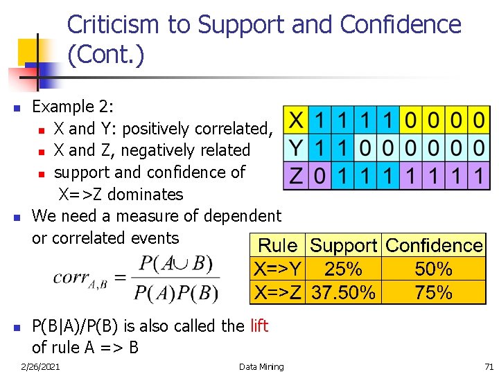
Criticism to Support and Confidence (Cont. ) n n n Example 2: n X and Y: positively correlated, n X and Z, negatively related n support and confidence of X=>Z dominates We need a measure of dependent or correlated events P(B|A)/P(B) is also called the lift of rule A => B 2/26/2021 Data Mining 71

Mining Association Rules in Large Databases n Association rule mining n Algorithms for scalable mining of (single-dimensional Boolean) association rules in transactional databases n Mining various kinds of association/correlation rules n Applications/extensions of frequent pattern mining n Summary 2/26/2021 Data Mining 72

Sequence Databases and Sequential Pattern Analysis n Transaction databases, time-series databases vs. sequence databases n Frequent patterns vs. (frequent) sequential patterns n Applications of sequential pattern mining n Customer shopping sequences: n n First buy computer, then CD-ROM, and then digital camera, within 3 months. Medical treatment, natural disasters (e. g. , earthquakes), science & engineering processes, stocks and markets, etc. n Telephone calling patterns, Weblog click streams n DNA sequences and gene structures 2/26/2021 Data Mining 73

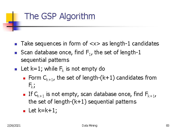
The GSP Algorithm n n n Take sequences in form of <x> as length-1 candidates Scan database once, find F 1, the set of length-1 sequential patterns Let k=1; while Fk is not empty do n n n 2/26/2021 Form Ck+1, the set of length-(k+1) candidates from F k; If Ck+1 is not empty, scan database once, find Fk+1, the set of length-(k+1) sequential patterns Let k=k+1; Data Mining 83

Mining Association Rules in Large Databases n Association rule mining n Algorithms for scalable mining of (single-dimensional Boolean) association rules in transactional databases n Mining various kinds of association/correlation rules n Applications/extensions of frequent pattern mining n Summary 2/26/2021 Data Mining 89

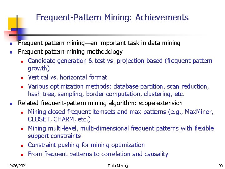
Frequent-Pattern Mining: Achievements n n n Frequent pattern mining—an important task in data mining Frequent pattern mining methodology n Candidate generation & test vs. projection-based (frequent-pattern growth) n Vertical vs. horizontal format n Various optimization methods: database partition, scan reduction, hash tree, sampling, border computation, clustering, etc. Related frequent-pattern mining algorithm: scope extension n Mining closed frequent itemsets and max-patterns (e. g. , Max. Miner, CLOSET, CHARM, etc. ) n Mining multi-level, multi-dimensional frequent patterns with flexible support constraints n Constraint pushing for mining optimization n From frequent patterns to correlation and causality 2/26/2021 Data Mining 90

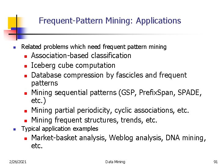
Frequent-Pattern Mining: Applications n Related problems which need frequent pattern mining n n n n Association-based classification Iceberg cube computation Database compression by fascicles and frequent patterns Mining sequential patterns (GSP, Prefix. Span, SPADE, etc. ) Mining partial periodicity, cyclic associations, etc. Mining frequent structures, trends, etc. Typical application examples n 2/26/2021 Market-basket analysis, Weblog analysis, DNA mining, etc. Data Mining 91

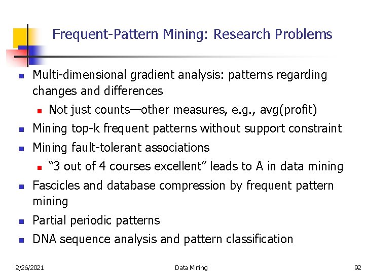
Frequent-Pattern Mining: Research Problems n Multi-dimensional gradient analysis: patterns regarding changes and differences n Not just counts—other measures, e. g. , avg(profit) n Mining top-k frequent patterns without support constraint n Mining fault-tolerant associations n n “ 3 out of 4 courses excellent” leads to A in data mining Fascicles and database compression by frequent pattern mining n Partial periodic patterns n DNA sequence analysis and pattern classification 2/26/2021 Data Mining 92