CS271 P Final Review Propositional Logic 7 1

CS-271 P Final Review • Propositional Logic • (7. 1 -7. 5) • First-Order Logic, Knowledge Representation • (8. 1 -8. 5, 9. 1 -9. 2) • Constraint Satisfaction Problems • (6. 1 -6. 4, except 6. 3) • Machine Learning • (18. 1 -18. 4) • Questions on any topic • Pre-mid-term material if time and class interest • Please review your quizzes, mid-term, & old tests • At least one question from a prior quiz or test will appear on the Final Exam (and all other tests)

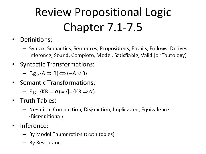
Review Propositional Logic Chapter 7. 1 -7. 5 • Definitions: – Syntax, Semantics, Sentences, Propositions, Entails, Follows, Derives, Inference, Sound, Complete, Model, Satisfiable, Valid (or Tautology) • Syntactic Transformations: – E. g. , (A B) ( A B) • Semantic Transformations: – E. g. , (KB |= ) (|= (KB ) • Truth Tables: – Negation, Conjunction, Disjunction, Implication, Equivalence (Biconditional) • Inference: – By Model Enumeration (truth tables) – By Resolution

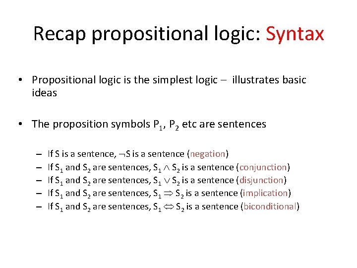
Recap propositional logic: Syntax • Propositional logic is the simplest logic – illustrates basic ideas • The proposition symbols P 1, P 2 etc are sentences – – – If S is a sentence, S is a sentence (negation) If S 1 and S 2 are sentences, S 1 S 2 is a sentence (conjunction) If S 1 and S 2 are sentences, S 1 S 2 is a sentence (disjunction) If S 1 and S 2 are sentences, S 1 S 2 is a sentence (implication) If S 1 and S 2 are sentences, S 1 S 2 is a sentence (biconditional)

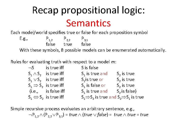
Recap propositional logic: Semantics Each model/world specifies true or false for each proposition symbol E. g. , P 1, 2 P 2, 2 P 3, 1 false true false With these symbols, 8 possible models can be enumerated automatically. Rules for evaluating truth with respect to a model m: S is true iff S is false S 1 S 2 is true iff S 1 is true and S 2 is true S 1 S 2 is true iff S 1 is true or S 2 is true S 1 S 2 is true iff S 1 is false or S 2 is true (i. e. , is false iff S 1 is true and S 2 is false) S 1 S 2 is true iff S 1 S 2 is true and S 2 S 1 is true Simple recursive process evaluates an arbitrary sentence, e. g. , P 1, 2 (P 2, 2 P 3, 1) = true (true false) = true

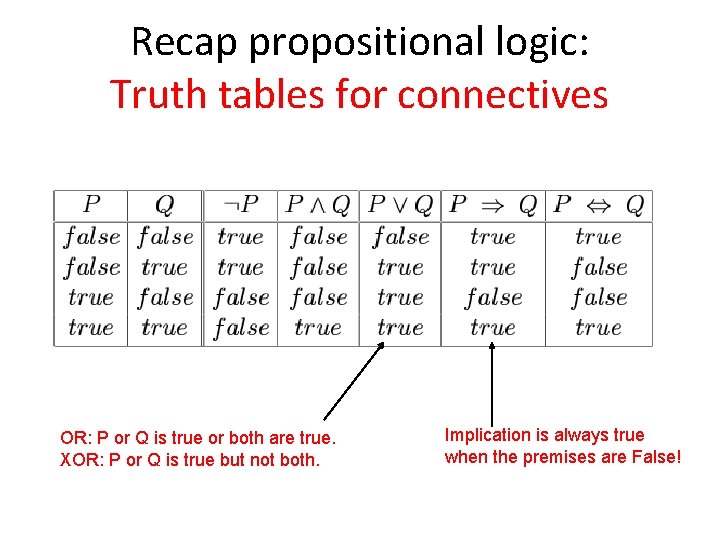
Recap propositional logic: Truth tables for connectives OR: P or Q is true or both are true. XOR: P or Q is true but not both. Implication is always true when the premises are False!

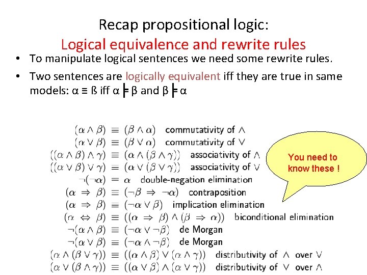
Recap propositional logic: Logical equivalence and rewrite rules • To manipulate logical sentences we need some rewrite rules. • Two sentences are logically equivalent iff they are true in same models: α ≡ ß iff α╞ β and β╞ α You need to know these !

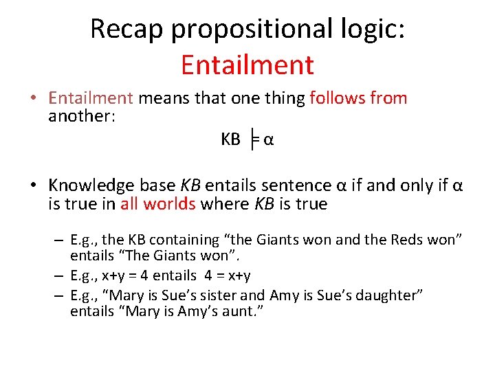
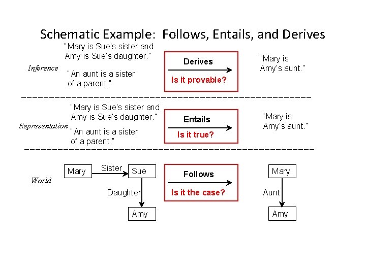
Recap propositional logic: Entailment • Entailment means that one thing follows from another: KB ╞ α • Knowledge base KB entails sentence α if and only if α is true in all worlds where KB is true – E. g. , the KB containing “the Giants won and the Reds won” entails “The Giants won”. – E. g. , x+y = 4 entails 4 = x+y – E. g. , “Mary is Sue’s sister and Amy is Sue’s daughter” entails “Mary is Amy’s aunt. ”

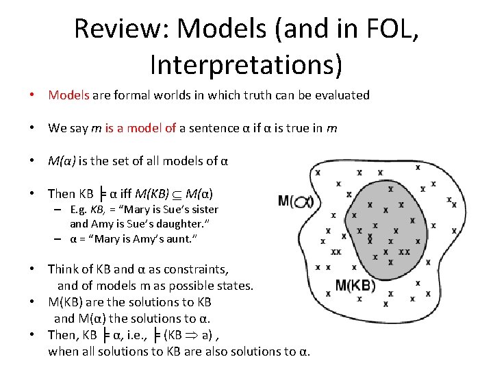
Review: Models (and in FOL, Interpretations) • Models are formal worlds in which truth can be evaluated • We say m is a model of a sentence α if α is true in m • M(α) is the set of all models of α • Then KB ╞ α iff M(KB) M(α) – E. g. KB, = “Mary is Sue’s sister and Amy is Sue’s daughter. ” – α = “Mary is Amy’s aunt. ” • Think of KB and α as constraints, and of models m as possible states. • M(KB) are the solutions to KB and M(α) the solutions to α. • Then, KB ╞ α, i. e. , ╞ (KB a) , when all solutions to KB are also solutions to α.

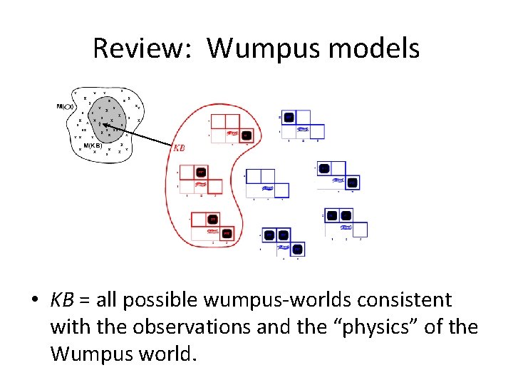
Review: Wumpus models • KB = all possible wumpus-worlds consistent with the observations and the “physics” of the Wumpus world.

Review: Wumpus models α 1 = "[1, 2] is safe", KB ╞ α 1, proved by model checking. Every model that makes KB true also makes α 1 true.

Wumpus models α 2 = "[2, 2] is safe", KB ╞ α 2

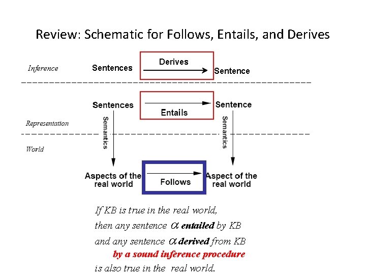
Review: Schematic for Follows, Entails, and Derives Inference Sentences Derives Sentence If KB is true in the real world, then any sentence entailed by KB and any sentence derived from KB by a sound inference procedure is also true in the real world.

Schematic Example: Follows, Entails, and Derives “Mary is Sue’s sister and Amy is Sue’s daughter. ” Inference “An aunt is a sister of a parent. ” Representation “Mary is Sue’s sister and Amy is Sue’s daughter. ” “An aunt is a sister of a parent. ” Mary Sister Sue World Daughter Amy Derives “Mary is Amy’s aunt. ” Is it provable? Entails Is it true? Follows Is it the case? “Mary is Amy’s aunt. ” Mary Aunt Amy

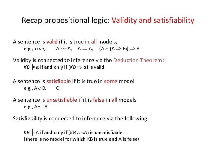
Recap propositional logic: Validity and satisfiability A sentence is valid if it is true in all models, e. g. , True, A A, (A B)) B Validity is connected to inference via the Deduction Theorem: KB ╞ α if and only if (KB α) is valid A sentence is satisfiable if it is true in some model e. g. , A B, C A sentence is unsatisfiable if it is false in all models e. g. , A A Satisfiability is connected to inference via the following: KB ╞ A if and only if (KB A) is unsatisfiable (there is no model for which KB is true and A is false)

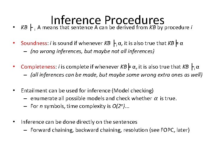
• KB ├ i Inference Procedures A means that sentence A can be derived from KB by procedure i • Soundness: i is sound if whenever KB ├i α, it is also true that KB╞ α – (no wrong inferences, but maybe not all inferences) • Completeness: i is complete if whenever KB╞ α, it is also true that KB ├i α – (all inferences can be made, but maybe some wrong extra ones as well) • Entailment can be used for inference (Model checking) – enumerate all possible models and check whether is true. – For n symbols, time complexity is O(2 n). . . • Inference can be done directly on the sentences – Forward chaining, backward chaining, resolution (see FOPC, later)

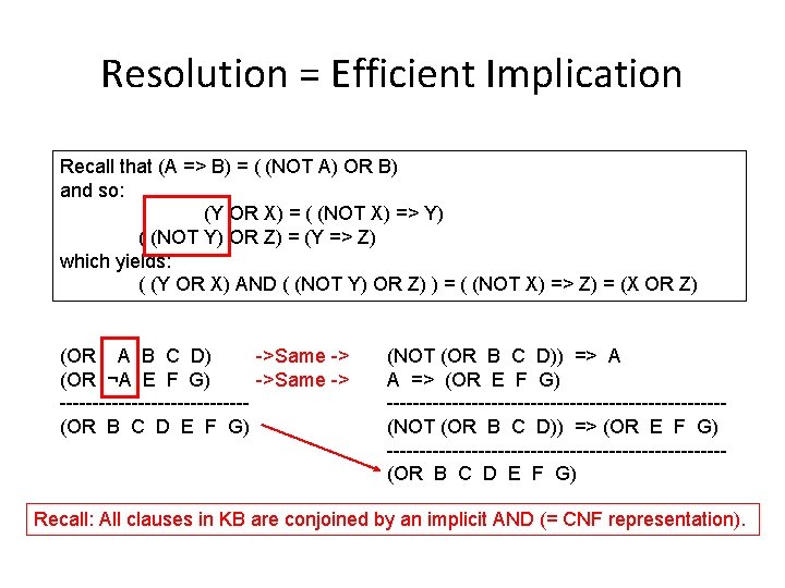
Resolution = Efficient Implication Recall that (A => B) = ( (NOT A) OR B) and so: (Y OR X) = ( (NOT X) => Y) ( (NOT Y) OR Z) = (Y => Z) which yields: ( (Y OR X) AND ( (NOT Y) OR Z) ) = ( (NOT X) => Z) = (X OR Z) ->Same -> (OR A B C D) ->Same -> (OR ¬A E F G) --------------(OR B C D E F G) (NOT (OR B C D)) => A A => (OR E F G) --------------------------(NOT (OR B C D)) => (OR E F G) --------------------------(OR B C D E F G) Recall: All clauses in KB are conjoined by an implicit AND (= CNF representation).

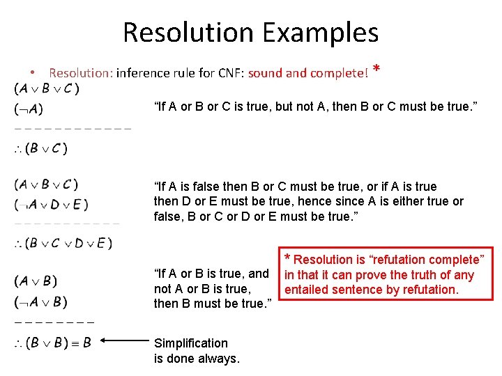
Resolution Examples • Resolution: inference rule for CNF: sound and complete! * “If A or B or C is true, but not A, then B or C must be true. ” “If A is false then B or C must be true, or if A is true then D or E must be true, hence since A is either true or false, B or C or D or E must be true. ” “If A or B is true, and not A or B is true, then B must be true. ” Simplification is done always. * Resolution is “refutation complete” in that it can prove the truth of any entailed sentence by refutation.

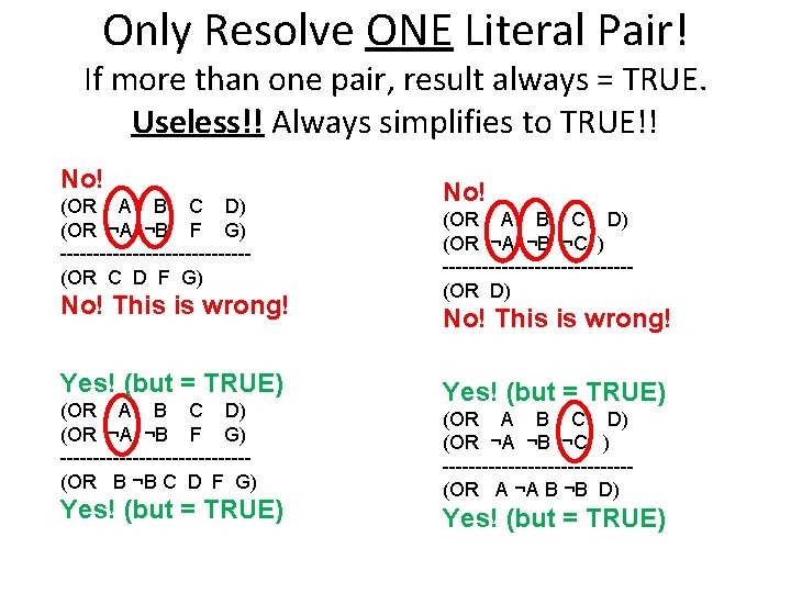
Only Resolve ONE Literal Pair! If more than one pair, result always = TRUE. Useless!! Always simplifies to TRUE!! No! (OR A B C D) (OR ¬A ¬B F G) --------------(OR C D F G) No! This is wrong! Yes! (but = TRUE) (OR A B C D) (OR ¬A ¬B F G) --------------(OR B ¬B C D F G) Yes! (but = TRUE) No! (OR A B C D) (OR ¬A ¬B ¬C ) --------------(OR D) No! This is wrong! Yes! (but = TRUE) (OR A B C D) (OR ¬A ¬B ¬C ) --------------(OR A ¬A B ¬B D) Yes! (but = TRUE)

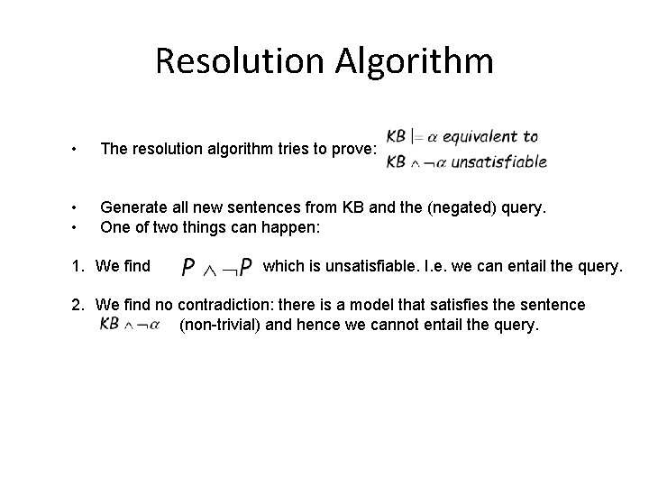
Resolution Algorithm • The resolution algorithm tries to prove: • • Generate all new sentences from KB and the (negated) query. One of two things can happen: 1. We find which is unsatisfiable. I. e. we can entail the query. 2. We find no contradiction: there is a model that satisfies the sentence (non-trivial) and hence we cannot entail the query.

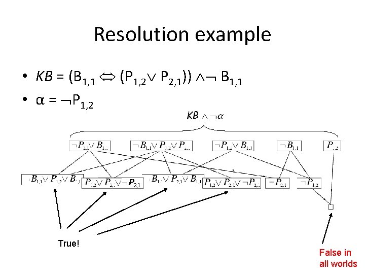
Resolution example • KB = (B 1, 1 (P 1, 2 P 2, 1)) B 1, 1 • α = P 1, 2 P 2, 1 True! False in all worlds

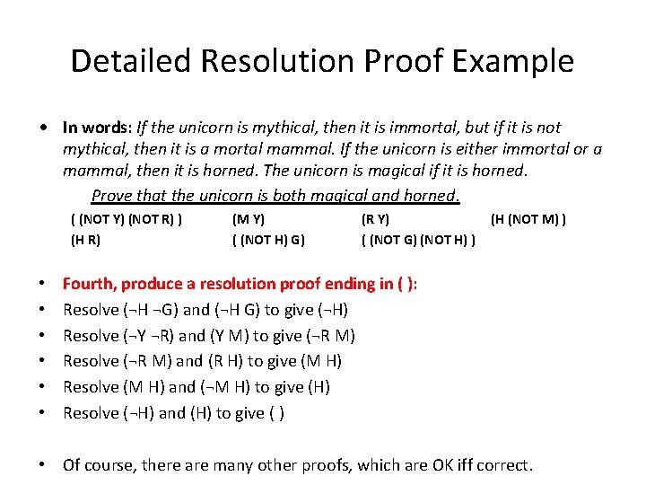
Detailed Resolution Proof Example • In words: If the unicorn is mythical, then it is immortal, but if it is not mythical, then it is a mortal mammal. If the unicorn is either immortal or a mammal, then it is horned. The unicorn is magical if it is horned. Prove that the unicorn is both magical and horned. ( (NOT Y) (NOT R) ) (H R) • • • (M Y) ( (NOT H) G) (R Y) ( (NOT G) (NOT H) ) (H (NOT M) ) Fourth, produce a resolution proof ending in ( ): Resolve (¬H ¬G) and (¬H G) to give (¬H) Resolve (¬Y ¬R) and (Y M) to give (¬R M) Resolve (¬R M) and (R H) to give (M H) Resolve (M H) and (¬M H) to give (H) Resolve (¬H) and (H) to give ( ) • Of course, there are many other proofs, which are OK iff correct.

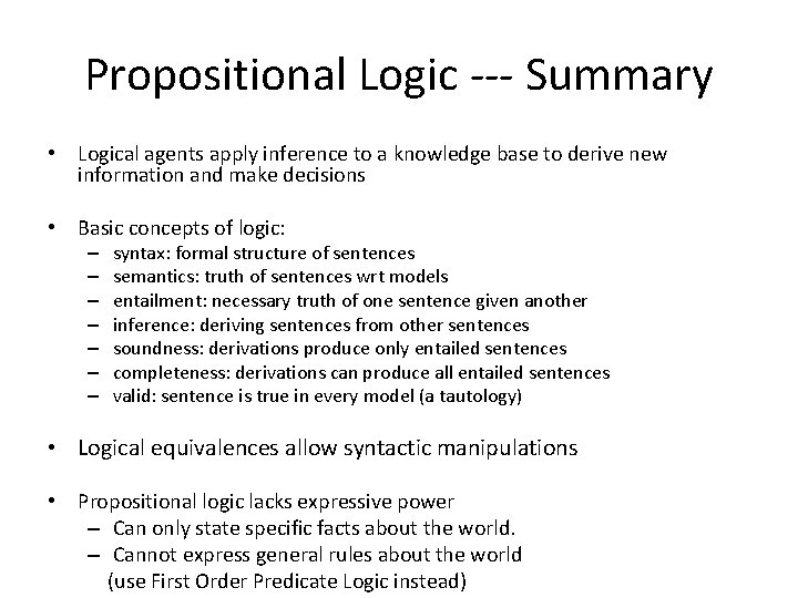
Propositional Logic --- Summary • Logical agents apply inference to a knowledge base to derive new information and make decisions • Basic concepts of logic: – – – – syntax: formal structure of sentences semantics: truth of sentences wrt models entailment: necessary truth of one sentence given another inference: deriving sentences from other sentences soundness: derivations produce only entailed sentences completeness: derivations can produce all entailed sentences valid: sentence is true in every model (a tautology) • Logical equivalences allow syntactic manipulations • Propositional logic lacks expressive power – Can only state specific facts about the world. – Cannot express general rules about the world (use First Order Predicate Logic instead)

CS-271 P Final Review • Propositional Logic • (7. 1 -7. 5) • First-Order Logic, Knowledge Representation • (8. 1 -8. 5, 9. 1 -9. 2) • Constraint Satisfaction Problems • (6. 1 -6. 4, except 6. 3) • Machine Learning • (18. 1 -18. 4) • Questions on any topic • Pre-mid-term material if time and class interest • Please review your quizzes, mid-term, & old tests • At least one question from a prior quiz or test will appear on the Final Exam (and all other tests)

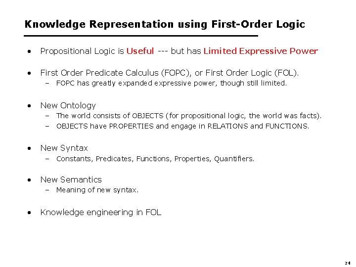
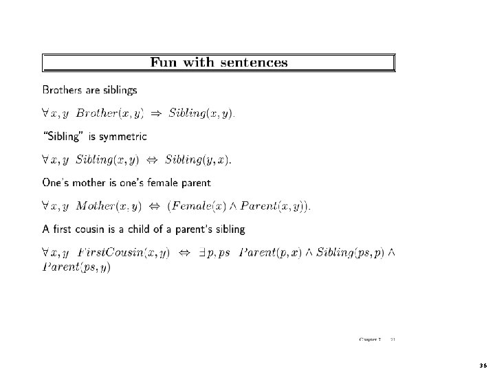
Knowledge Representation using First-Order Logic • Propositional Logic is Useful --- but has Limited Expressive Power • First Order Predicate Calculus (FOPC), or First Order Logic (FOL). – FOPC has greatly expanded expressive power, though still limited. • New Ontology – The world consists of OBJECTS (for propositional logic, the world was facts). – OBJECTS have PROPERTIES and engage in RELATIONS and FUNCTIONS. • New Syntax – Constants, Predicates, Functions, Properties, Quantifiers. • New Semantics – Meaning of new syntax. • Knowledge engineering in FOL 24

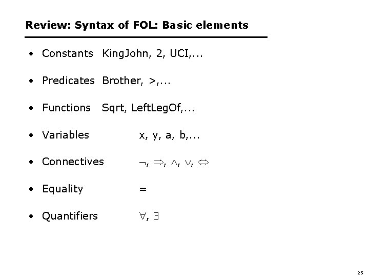
Review: Syntax of FOL: Basic elements • Constants King. John, 2, UCI, . . . • Predicates Brother, >, . . . • Functions Sqrt, Left. Leg. Of, . . . • Variables x, y, a, b, . . . • Connectives , , • Equality = • Quantifiers , 25

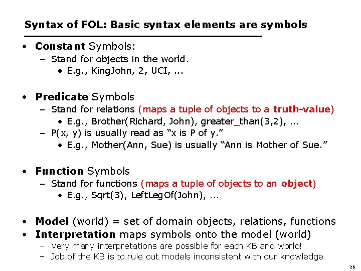
Syntax of FOL: Basic syntax elements are symbols • Constant Symbols: – Stand for objects in the world. • E. g. , King. John, 2, UCI, . . . • Predicate Symbols – Stand for relations (maps a tuple of objects to a truth-value) • E. g. , Brother(Richard, John), greater_than(3, 2), . . . – P(x, y) is usually read as “x is P of y. ” • E. g. , Mother(Ann, Sue) is usually “Ann is Mother of Sue. ” • Function Symbols – Stand for functions (maps a tuple of objects to an object) • E. g. , Sqrt(3), Left. Leg. Of(John), . . . • Model (world) = set of domain objects, relations, functions • Interpretation maps symbols onto the model (world) – Very many interpretations are possible for each KB and world! – Job of the KB is to rule out models inconsistent with our knowledge. 26

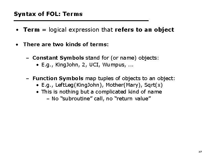
Syntax of FOL: Terms • Term = logical expression that refers to an object • There are two kinds of terms: – Constant Symbols stand for (or name) objects: • E. g. , King. John, 2, UCI, Wumpus, . . . – Function Symbols map tuples of objects to an object: • E. g. , Left. Leg(King. John), Mother(Mary), Sqrt(x) • This is nothing but a complicated kind of name – No “subroutine” call, no “return value” 27

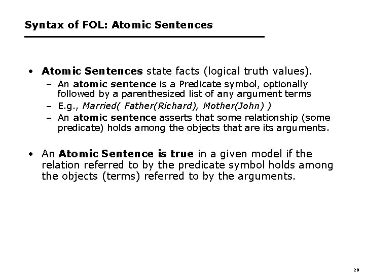
Syntax of FOL: Atomic Sentences • Atomic Sentences state facts (logical truth values). – An atomic sentence is a Predicate symbol, optionally followed by a parenthesized list of any argument terms – E. g. , Married( Father(Richard), Mother(John) ) – An atomic sentence asserts that some relationship (some predicate) holds among the objects that are its arguments. • An Atomic Sentence is true in a given model if the relation referred to by the predicate symbol holds among the objects (terms) referred to by the arguments. 28

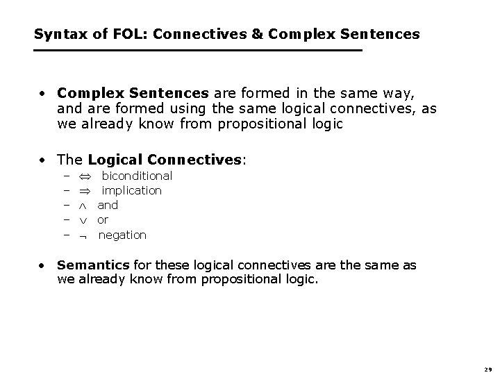
Syntax of FOL: Connectives & Complex Sentences • Complex Sentences are formed in the same way, and are formed using the same logical connectives, as we already know from propositional logic • The Logical Connectives: – – – biconditional implication and or negation • Semantics for these logical connectives are the same as we already know from propositional logic. 29

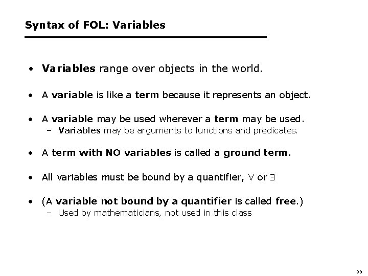
Syntax of FOL: Variables • Variables range over objects in the world. • A variable is like a term because it represents an object. • A variable may be used wherever a term may be used. – Variables may be arguments to functions and predicates. • A term with NO variables is called a ground term. • All variables must be bound by a quantifier, or • (A variable not bound by a quantifier is called free. ) – Used by mathematicians, not used in this class 30

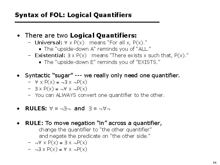
Syntax of FOL: Logical Quantifiers • There are two Logical Quantifiers: – Universal: x P(x) means “For all x, P(x). ” • The “upside-down A” reminds you of “ALL. ” – Existential: x P(x) means “There exists x such that, P(x). ” • The “upside-down E” reminds you of “EXISTS. ” • Syntactic “sugar” --- we really only need one quantifier. – x P(x) – You can ALWAYS convert one quantifier to the other. • RULES: and • RULE: To move negation “in” across a quantifier, change the quantifier to “the other quantifier” and negate the predicate on “the other side. ” – x P(x) 31

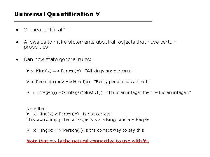
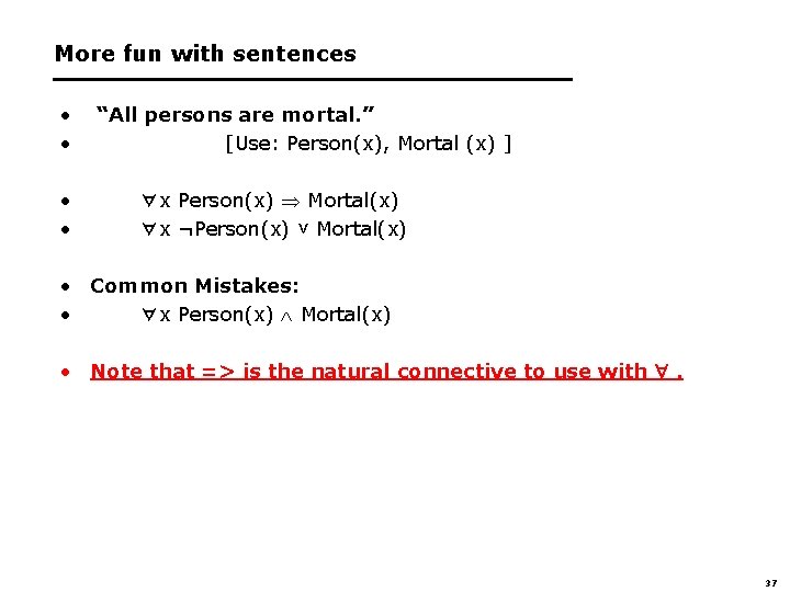
Universal Quantification • means “for all” • Allows us to make statements about all objects that have certain properties • Can now state general rules: x King(x) => Person(x) “All kings are persons. ” x Person(x) => Has. Head(x) “Every person has a head. ” i Integer(i) => Integer(plus(i, 1)) “If i is an integer then i+1 is an integer. ” Note that x King(x) Person(x) is not correct! This would imply that all objects x are Kings and are People x King(x) => Person(x) is the correct way to say this Note that => is the natural connective to use with .

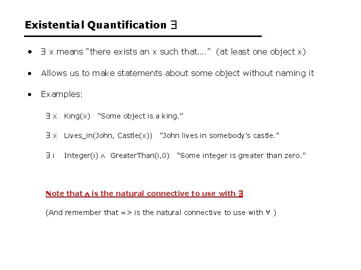
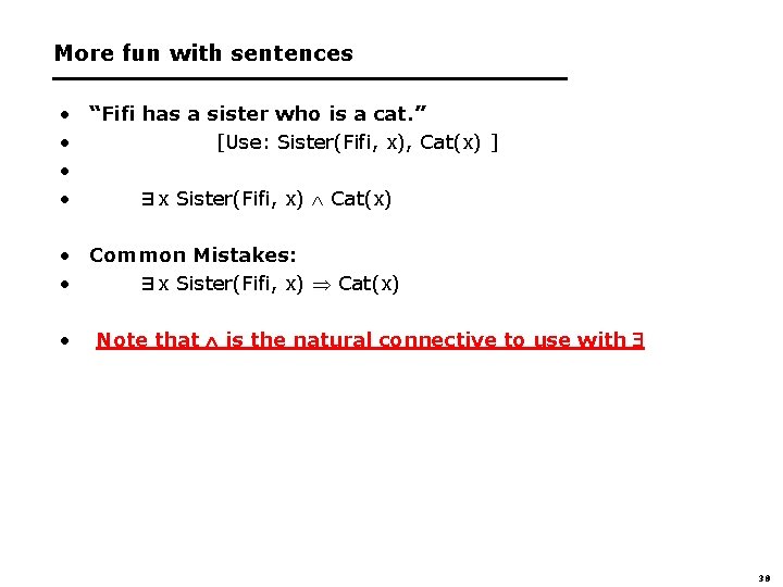
Existential Quantification • x means “there exists an x such that…. ” (at least one object x) • Allows us to make statements about some object without naming it • Examples: x King(x) “Some object is a king. ” x Lives_in(John, Castle(x)) “John lives in somebody’s castle. ” i Integer(i) Greater. Than(i, 0) “Some integer is greater than zero. ” Note that is the natural connective to use with (And remember that => is the natural connective to use with )

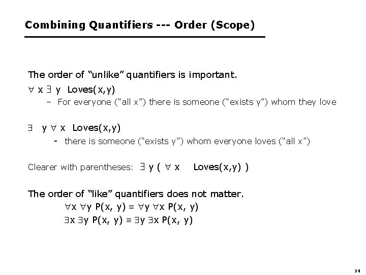
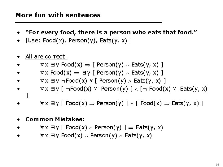
Combining Quantifiers --- Order (Scope) The order of “unlike” quantifiers is important. x y Loves(x, y) – For everyone (“all x”) there is someone (“exists y”) whom they love y x Loves(x, y) - there is someone (“exists y”) whom everyone loves (“all x”) Clearer with parentheses: y ( x Loves(x, y) ) The order of “like” quantifiers does not matter. x y P(x, y) y x P(x, y) 34

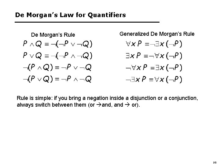
De Morgan’s Law for Quantifiers De Morgan’s Rule Generalized De Morgan’s Rule is simple: if you bring a negation inside a disjunction or a conjunction, always switch between them (or and, and or). 35

36

More fun with sentences • • “All persons are mortal. ” [Use: Person(x), Mortal (x) ] ∀x Person(x) Mortal(x) ∀x ¬Person(x) ˅ Mortal(x) • Common Mistakes: • ∀x Person(x) Mortal(x) • Note that => is the natural connective to use with . 37

More fun with sentences • “Fifi has a sister who is a cat. ” • [Use: Sister(Fifi, x), Cat(x) ] • • ∃x Sister(Fifi, x) Cat(x) • Common Mistakes: • ∃x Sister(Fifi, x) Cat(x) • Note that is the natural connective to use with 38

More fun with sentences • “For every food, there is a person who eats that food. ” • [Use: Food(x), Person(y), Eats(y, x) ] • All are correct: • ∀x ∃y Food(x) [ Person(y) Eats(y, x) ] • ∀x Food(x) ∃y [ Person(y) Eats(y, x) ] • ∀x ∃y ¬Food(x) ˅ [ Person(y) Eats(y, x) ] • ∀x ∃y [ ¬Food(x) ˅ Person(y) ] [¬ Food(x) ˅ Eats(y, x) ] • ∀x ∃y [ Food(x) Person(y) ] [ Food(x) Eats(y, x) ] • Common Mistakes: • ∀x ∃y [ Food(x) Person(y) ] Eats(y, x) • ∀x ∃y Food(x) Person(y) Eats(y, x) 39

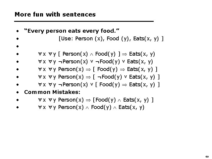
More fun with sentences • “Every person eats every food. ” • [Use: Person (x), Food (y), Eats(x, y) ] • • ∀x ∀y [ Person(x) Food(y) ] Eats(x, y) • ∀x ∀y ¬Person(x) ˅ ¬Food(y) ˅ Eats(x, y) • ∀x ∀y Person(x) [ Food(y) Eats(x, y) ] • ∀x ∀y Person(x) [ ¬Food(y) ˅ Eats(x, y) ] • ∀x ∀y ¬Person(x) ˅ [ Food(y) Eats(x, y) ] • Common Mistakes: • ∀x ∀y Person(x) [Food(y) Eats(x, y) ] • ∀x ∀y Person(x) Food(y) Eats(x, y) 40

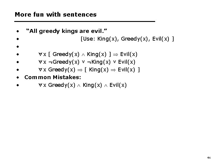
More fun with sentences • “All greedy kings are evil. ” • [Use: King(x), Greedy(x), Evil(x) ] • • ∀x [ Greedy(x) King(x) ] Evil(x) • ∀x ¬Greedy(x) ˅ ¬King(x) ˅ Evil(x) • ∀x Greedy(x) [ King(x) Evil(x) ] • Common Mistakes: • ∀x Greedy(x) King(x) Evil(x) 41

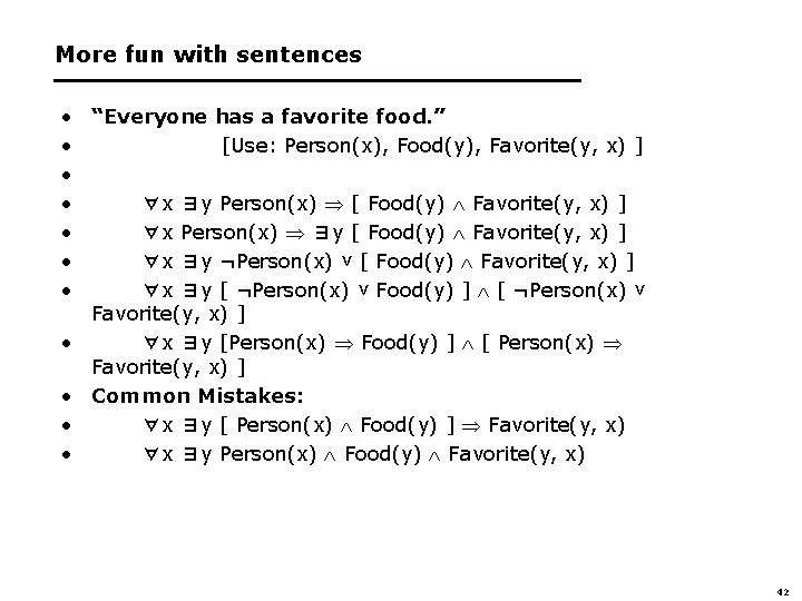
More fun with sentences • “Everyone has a favorite food. ” • [Use: Person(x), Food(y), Favorite(y, x) ] • • ∀x ∃y Person(x) [ Food(y) Favorite(y, x) ] • ∀x Person(x) ∃y [ Food(y) Favorite(y, x) ] • ∀x ∃y ¬Person(x) ˅ [ Food(y) Favorite(y, x) ] • ∀x ∃y [ ¬Person(x) ˅ Food(y) ] [ ¬Person(x) ˅ Favorite(y, x) ] • ∀x ∃y [Person(x) Food(y) ] [ Person(x) Favorite(y, x) ] • Common Mistakes: • ∀x ∃y [ Person(x) Food(y) ] Favorite(y, x) • ∀x ∃y Person(x) Food(y) Favorite(y, x) 42

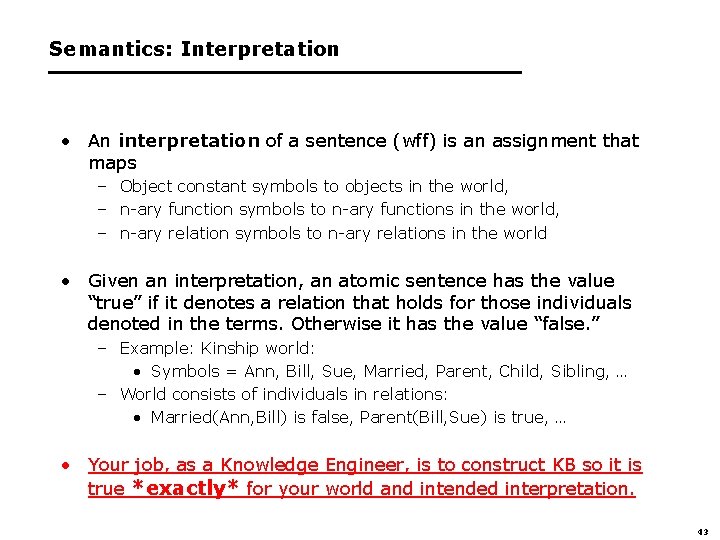
Semantics: Interpretation • An interpretation of a sentence (wff) is an assignment that maps – Object constant symbols to objects in the world, – n-ary function symbols to n-ary functions in the world, – n-ary relation symbols to n-ary relations in the world • Given an interpretation, an atomic sentence has the value “true” if it denotes a relation that holds for those individuals denoted in the terms. Otherwise it has the value “false. ” – Example: Kinship world: • Symbols = Ann, Bill, Sue, Married, Parent, Child, Sibling, … – World consists of individuals in relations: • Married(Ann, Bill) is false, Parent(Bill, Sue) is true, … • Your job, as a Knowledge Engineer, is to construct KB so it is true *exactly* for your world and intended interpretation. 43

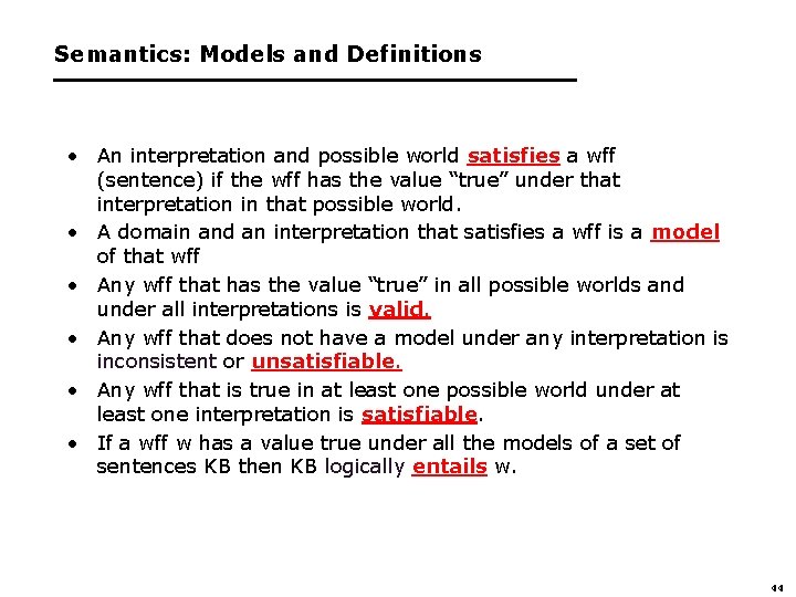
Semantics: Models and Definitions • An interpretation and possible world satisfies a wff (sentence) if the wff has the value “true” under that interpretation in that possible world. • A domain and an interpretation that satisfies a wff is a model of that wff • Any wff that has the value “true” in all possible worlds and under all interpretations is valid. • Any wff that does not have a model under any interpretation is inconsistent or unsatisfiable. • Any wff that is true in at least one possible world under at least one interpretation is satisfiable. • If a wff w has a value true under all the models of a set of sentences KB then KB logically entails w. 44

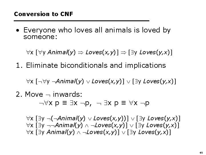
Conversion to CNF • Everyone who loves all animals is loved by someone: x [ y Animal(y) Loves(x, y)] [ y Loves(y, x)] 1. Eliminate biconditionals and implications x [ y Animal(y) Loves(x, y)] [ y Loves(y, x)] 2. Move inwards: x p ≡ x p, x p ≡ x p x [ y ( Animal(y) Loves(x, y))] [ y Loves(y, x)] x [ y Animal(y) Loves(x, y)] [ y Loves(y, x)] x [ y Animal(y) Loves(x, y)] [ y Loves(y, x)] 45

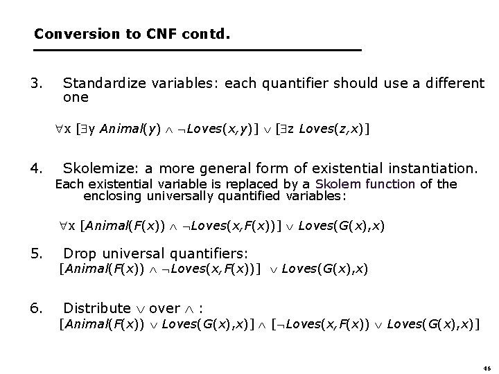
Conversion to CNF contd. 3. Standardize variables: each quantifier should use a different one x [ y Animal(y) Loves(x, y)] [ z Loves(z, x)] 4. Skolemize: a more general form of existential instantiation. Each existential variable is replaced by a Skolem function of the enclosing universally quantified variables: x [Animal(F(x)) Loves(x, F(x))] Loves(G(x), x) 5. 6. Drop universal quantifiers: [Animal(F(x)) Loves(x, F(x))] Loves(G(x), x) Distribute over : [Animal(F(x)) Loves(G(x), x)] [ Loves(x, F(x)) Loves(G(x), x)] 46

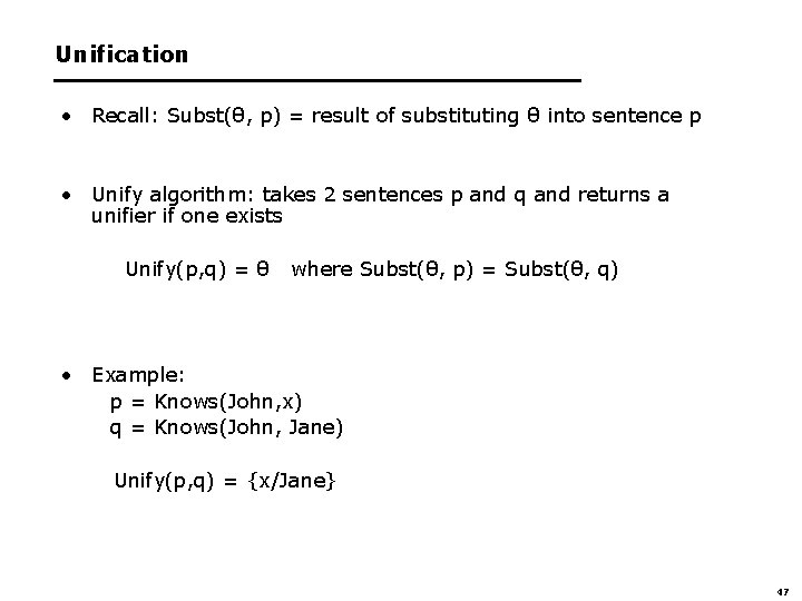
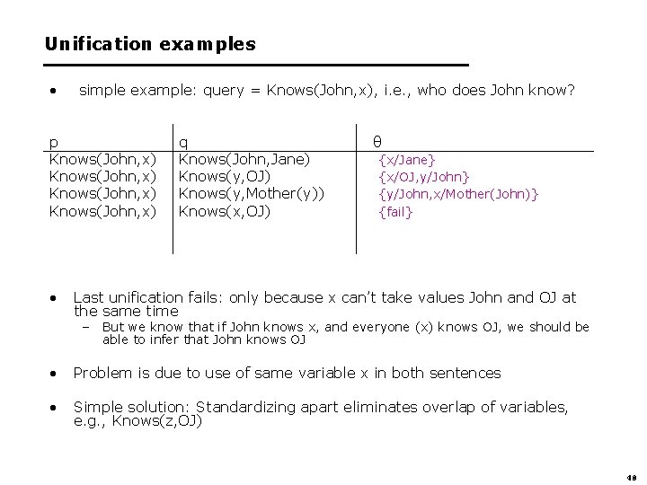
Unification • Recall: Subst(θ, p) = result of substituting θ into sentence p • Unify algorithm: takes 2 sentences p and q and returns a unifier if one exists Unify(p, q) = θ where Subst(θ, p) = Subst(θ, q) • Example: p = Knows(John, x) q = Knows(John, Jane) Unify(p, q) = {x/Jane} 47

Unification examples • simple example: query = Knows(John, x), i. e. , who does John know? p Knows(John, x) • q Knows(John, Jane) Knows(y, OJ) Knows(y, Mother(y)) Knows(x, OJ) θ {x/Jane} {x/OJ, y/John} {y/John, x/Mother(John)} {fail} Last unification fails: only because x can’t take values John and OJ at the same time – But we know that if John knows x, and everyone (x) knows OJ, we should be able to infer that John knows OJ • Problem is due to use of same variable x in both sentences • Simple solution: Standardizing apart eliminates overlap of variables, e. g. , Knows(z, OJ) 48

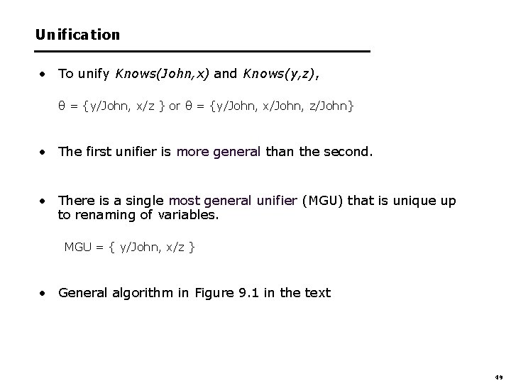
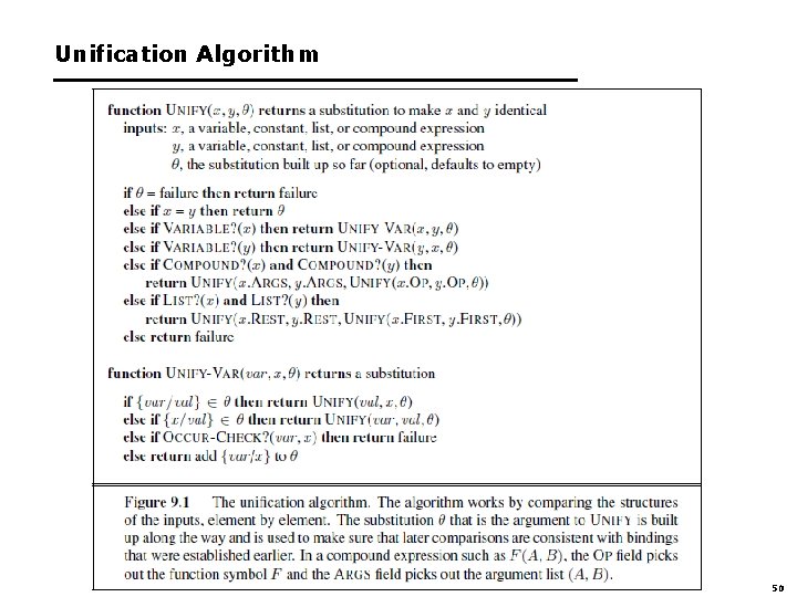
Unification • To unify Knows(John, x) and Knows(y, z), θ = {y/John, x/z } or θ = {y/John, x/John, z/John} • The first unifier is more general than the second. • There is a single most general unifier (MGU) that is unique up to renaming of variables. MGU = { y/John, x/z } • General algorithm in Figure 9. 1 in the text 49

Unification Algorithm 50

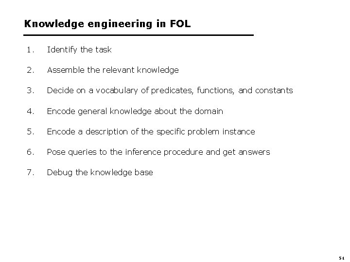
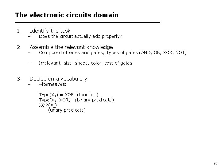
Knowledge engineering in FOL 1. Identify the task 2. Assemble the relevant knowledge 3. Decide on a vocabulary of predicates, functions, and constants 4. Encode general knowledge about the domain 5. Encode a description of the specific problem instance 6. Pose queries to the inference procedure and get answers 7. Debug the knowledge base 51

The electronic circuits domain 1. 2. 3. Identify the task – Does the circuit actually add properly? Assemble the relevant knowledge – Composed of wires and gates; Types of gates (AND, OR, XOR, NOT) – Irrelevant: size, shape, color, cost of gates Decide on a vocabulary – Alternatives: Type(X 1) = XOR (function) Type(X 1, XOR) (binary predicate) XOR(X 1) (unary predicate) 52

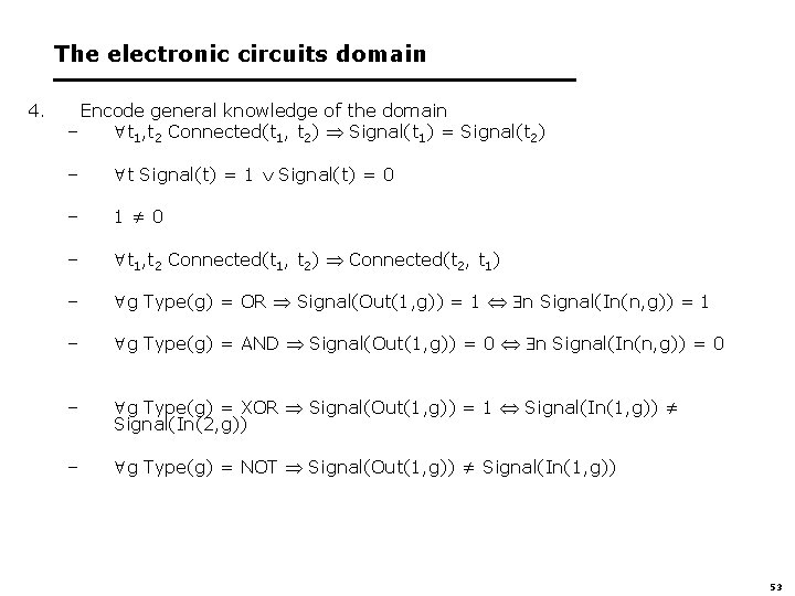
The electronic circuits domain 4. Encode general knowledge of the domain – t 1, t 2 Connected(t 1, t 2) Signal(t 1) = Signal(t 2) – t Signal(t) = 1 Signal(t) = 0 – 1 ≠ 0 – t 1, t 2 Connected(t 1, t 2) Connected(t 2, t 1) – g Type(g) = OR Signal(Out(1, g)) = 1 n Signal(In(n, g)) = 1 – g Type(g) = AND Signal(Out(1, g)) = 0 n Signal(In(n, g)) = 0 – g Type(g) = XOR Signal(Out(1, g)) = 1 Signal(In(1, g)) ≠ Signal(In(2, g)) – g Type(g) = NOT Signal(Out(1, g)) ≠ Signal(In(1, g)) 53

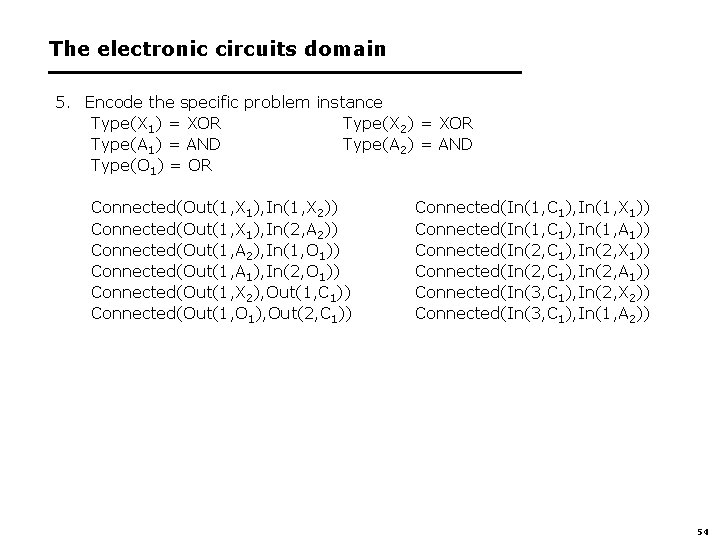
The electronic circuits domain 5. Encode the specific problem instance Type(X 1) = XOR Type(X 2) = XOR Type(A 1) = AND Type(A 2) = AND Type(O 1) = OR Connected(Out(1, X 1), In(1, X 2)) Connected(Out(1, X 1), In(2, A 2)) Connected(Out(1, A 2), In(1, O 1)) Connected(Out(1, A 1), In(2, O 1)) Connected(Out(1, X 2), Out(1, C 1)) Connected(Out(1, O 1), Out(2, C 1)) Connected(In(1, C 1), In(1, X 1)) Connected(In(1, C 1), In(1, A 1)) Connected(In(2, C 1), In(2, X 1)) Connected(In(2, C 1), In(2, A 1)) Connected(In(3, C 1), In(2, X 2)) Connected(In(3, C 1), In(1, A 2)) 54

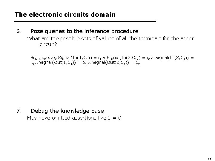
The electronic circuits domain 6. Pose queries to the inference procedure What are the possible sets of values of all the terminals for the adder circuit? i 1, i 2, i 3, o 1, o 2 Signal(In(1, C 1)) = i 1 Signal(In(2, C 1)) = i 2 Signal(In(3, C 1)) = i 3 Signal(Out(1, C 1)) = o 1 Signal(Out(2, C 1)) = o 2 7. Debug the knowledge base May have omitted assertions like 1 ≠ 0 55

CS-271 P Final Review • Propositional Logic • (7. 1 -7. 5) • First-Order Logic, Knowledge Representation • (8. 1 -8. 5, 9. 1 -9. 2) • Constraint Satisfaction Problems • (6. 1 -6. 4, except 6. 3) • Machine Learning • (18. 1 -18. 4) • Questions on any topic • Pre-mid-term material if time and class interest • Please review your quizzes, mid-term, & old tests • At least one question from a prior quiz or test will appear on the Final Exam (and all other tests) 56

Review Constraint Satisfaction Chapter 6. 1 -6. 4, except 6. 3. 3 • What is a CSP • Backtracking for CSP • Local search for CSPs

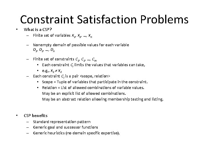
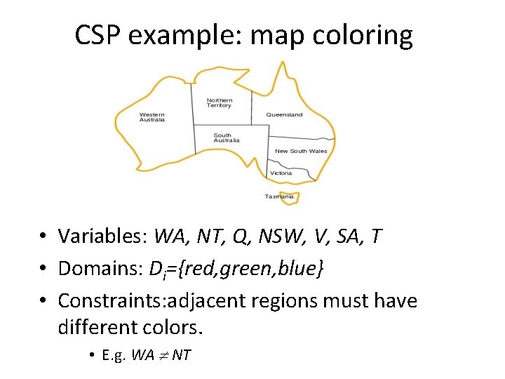
• Constraint Satisfaction Problems What is a CSP? – Finite set of variables X 1, X 2, …, Xn – Nonempty domain of possible values for each variable D 1, D 2, …, Dn – Finite set of constraints C 1, C 2, …, Cm • Each constraint Ci limits the values that variables can take, • e. g. , X 1 ≠ X 2 – Each constraint Ci is a pair <scope, relation> • Scope = Tuple of variables that participate in the constraint. • Relation = List of allowed combinations of variable values. May be an explicit list of allowed combinations. May be an abstract relation allowing membership testing and listing. • CSP benefits – Standard representation pattern – Generic goal and successor functions – Generic heuristics (no domain specific expertise).

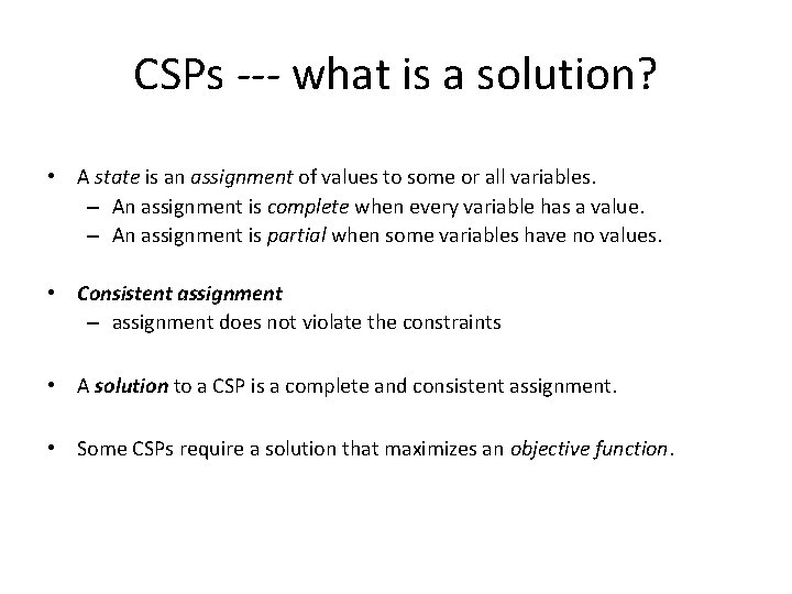
CSPs --- what is a solution? • A state is an assignment of values to some or all variables. – An assignment is complete when every variable has a value. – An assignment is partial when some variables have no values. • Consistent assignment – assignment does not violate the constraints • A solution to a CSP is a complete and consistent assignment. • Some CSPs require a solution that maximizes an objective function.

CSP example: map coloring • Variables: WA, NT, Q, NSW, V, SA, T • Domains: Di={red, green, blue} • Constraints: adjacent regions must have different colors. • E. g. WA NT

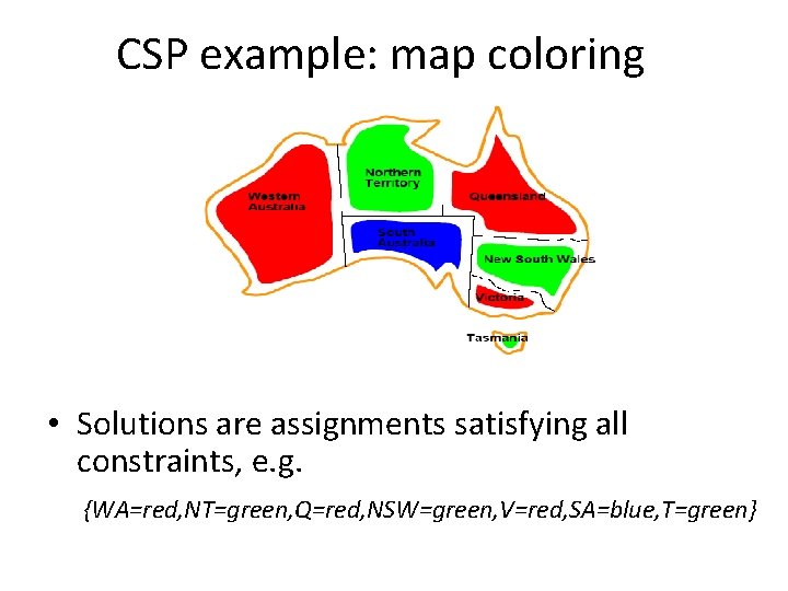
CSP example: map coloring • Solutions are assignments satisfying all constraints, e. g. {WA=red, NT=green, Q=red, NSW=green, V=red, SA=blue, T=green}

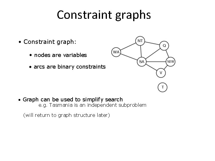
Constraint graphs • Constraint graph: • nodes are variables • arcs are binary constraints • Graph can be used to simplify search e. g. Tasmania is an independent subproblem (will return to graph structure later)

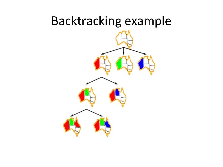
Backtracking example

Minimum remaining values (MRV) var SELECT-UNASSIGNED-VARIABLE(VARIABLES[csp], assignment, csp) • A. k. a. most constrained variable heuristic • Heuristic Rule: choose variable with the fewest legal moves – e. g. , will immediately detect failure if X has no legal values

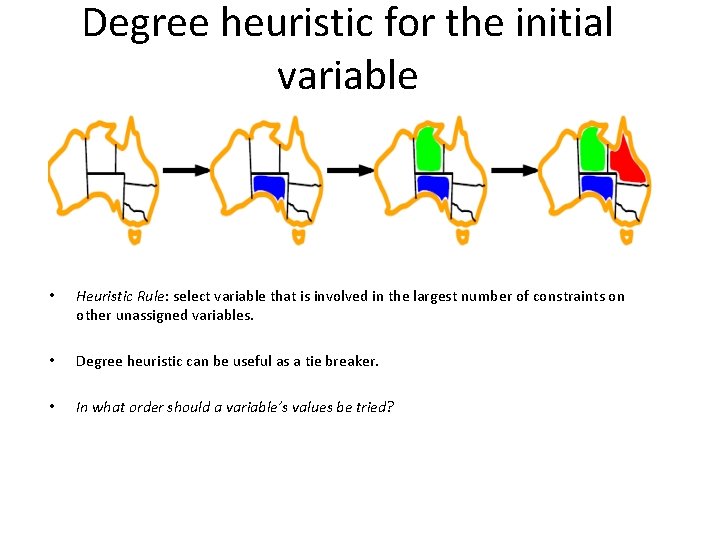
Degree heuristic for the initial variable • Heuristic Rule: select variable that is involved in the largest number of constraints on other unassigned variables. • Degree heuristic can be useful as a tie breaker. • In what order should a variable’s values be tried?

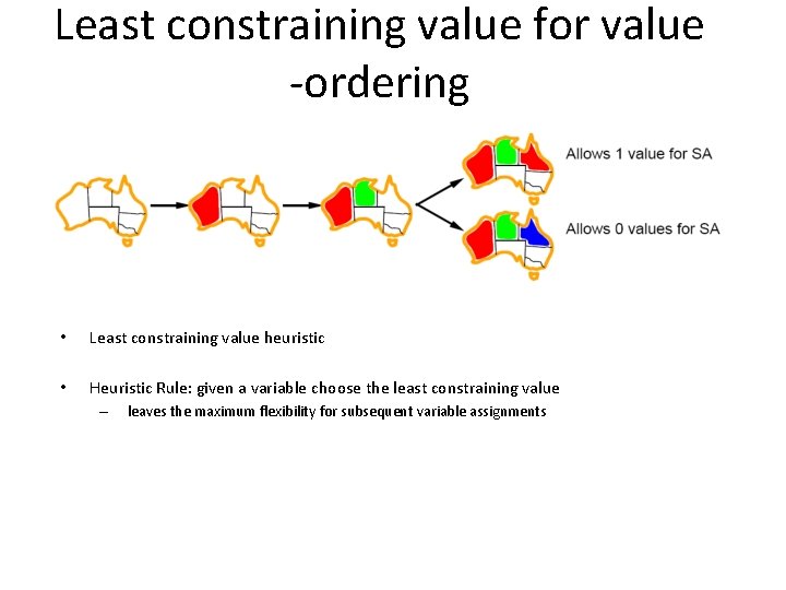
Least constraining value for value -ordering • Least constraining value heuristic • Heuristic Rule: given a variable choose the least constraining value – leaves the maximum flexibility for subsequent variable assignments

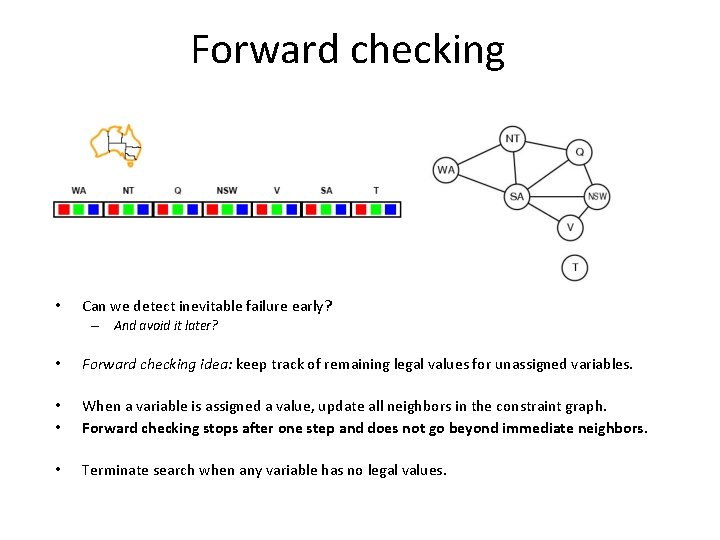
Forward checking • Can we detect inevitable failure early? – And avoid it later? • Forward checking idea: keep track of remaining legal values for unassigned variables. • • When a variable is assigned a value, update all neighbors in the constraint graph. Forward checking stops after one step and does not go beyond immediate neighbors. • Terminate search when any variable has no legal values.

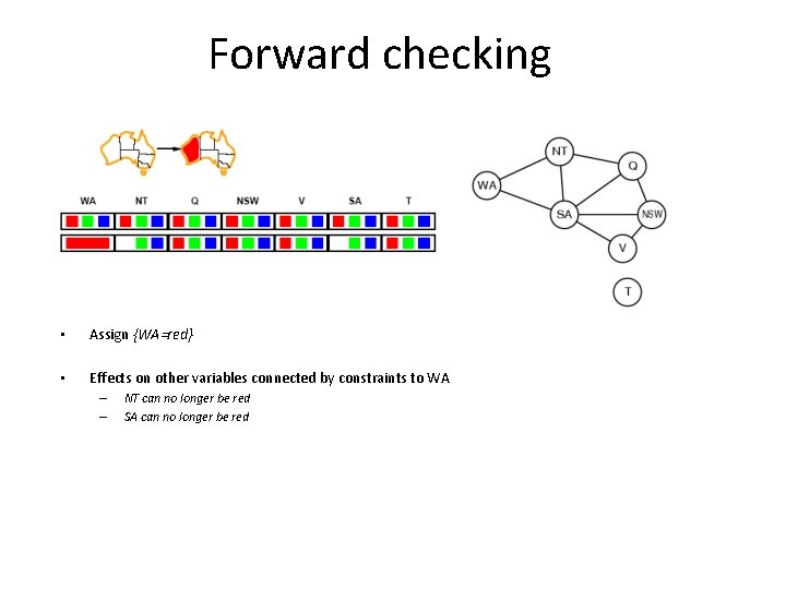
Forward checking • Assign {WA=red} • Effects on other variables connected by constraints to WA – – NT can no longer be red SA can no longer be red

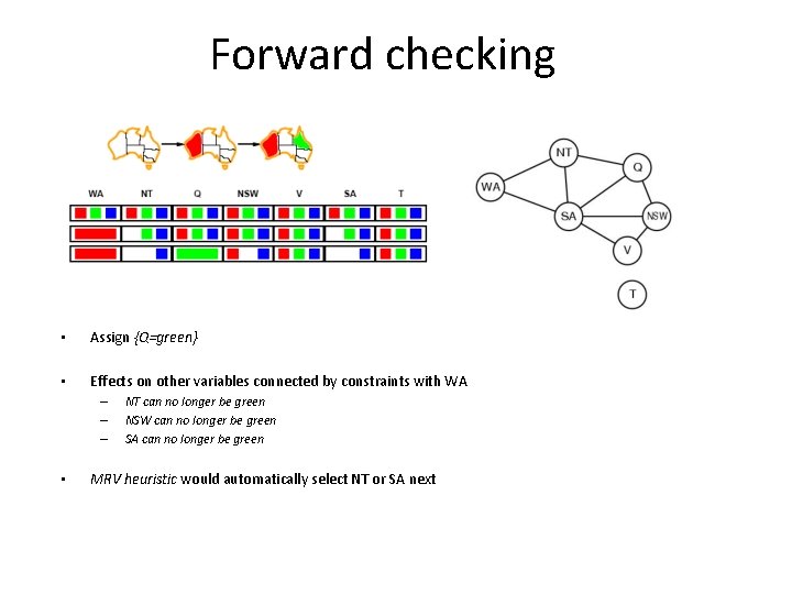
Forward checking • Assign {Q=green} • Effects on other variables connected by constraints with WA – – – • NT can no longer be green NSW can no longer be green SA can no longer be green MRV heuristic would automatically select NT or SA next

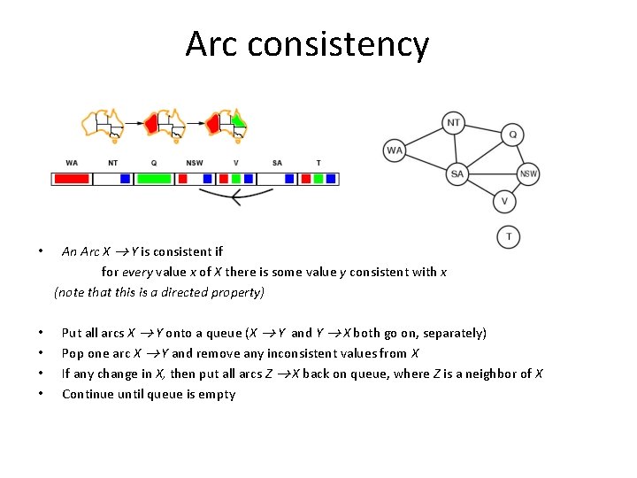
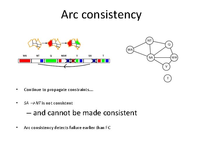
Arc consistency • • • An Arc X Y is consistent if for every value x of X there is some value y consistent with x (note that this is a directed property) Put all arcs X Y onto a queue (X Y and Y X both go on, separately) Pop one arc X Y and remove any inconsistent values from X If any change in X, then put all arcs Z X back on queue, where Z is a neighbor of X Continue until queue is empty

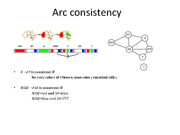
Arc consistency • X Y is consistent if for every value x of X there is some value y consistent with x • NSW SA is consistent if NSW=red and SA=blue NSW=blue and SA=? ? ?

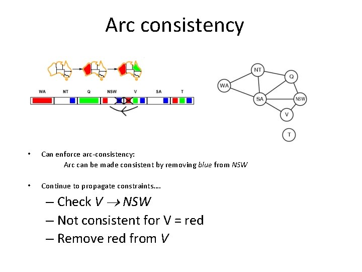
Arc consistency • Can enforce arc-consistency: Arc can be made consistent by removing blue from NSW • Continue to propagate constraints…. – Check V NSW – Not consistent for V = red – Remove red from V

Arc consistency • Continue to propagate constraints…. • SA NT is not consistent – and cannot be made consistent • Arc consistency detects failure earlier than FC

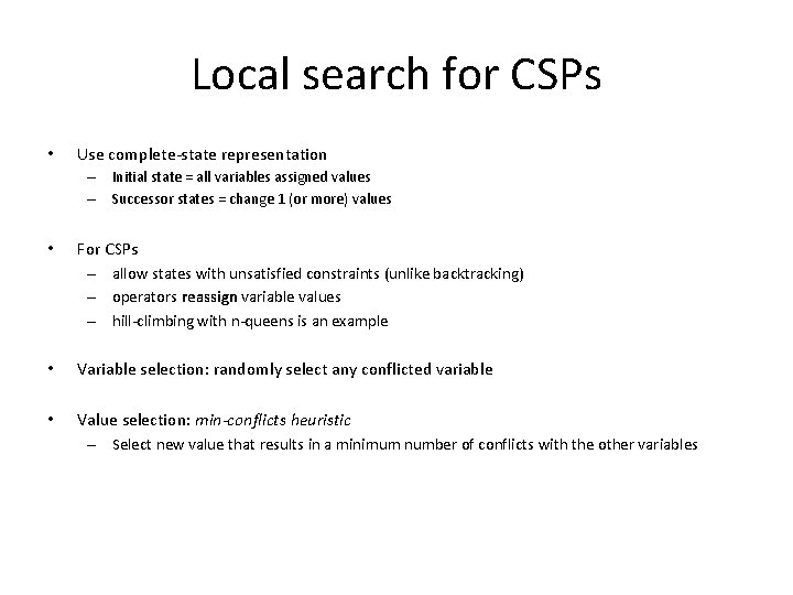
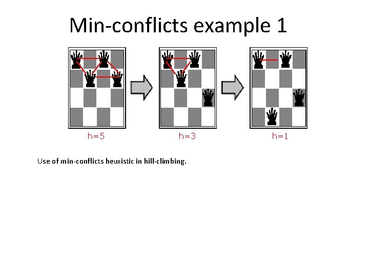
Local search for CSPs • Use complete-state representation – Initial state = all variables assigned values – Successor states = change 1 (or more) values • For CSPs – allow states with unsatisfied constraints (unlike backtracking) – operators reassign variable values – hill-climbing with n-queens is an example • Variable selection: randomly select any conflicted variable • Value selection: min-conflicts heuristic – Select new value that results in a minimum number of conflicts with the other variables

Min-conflicts example 1 h=5 h=3 Use of min-conflicts heuristic in hill-climbing. h=1

CS-271 P Final Review • Propositional Logic • (7. 1 -7. 5) • First-Order Logic, Knowledge Representation • (8. 1 -8. 5, 9. 1 -9. 2) • Constraint Satisfaction Problems • (6. 1 -6. 4, except 6. 3) • Machine Learning • (18. 1 -18. 4) • Questions on any topic • Pre-mid-term material if time and class interest • Please review your quizzes, mid-term, & old tests • At least one question from a prior quiz or test will appear on the Final Exam (and all other tests) 76

The importance of a good representation • Properties of a good representation: • • • Reveals important features Hides irrelevant detail Exposes useful constraints Makes frequent operations easy-to-do Supports local inferences from local features • • Called the “soda straw” principle or “locality” principle Inference from features “through a soda straw” • Rapidly or efficiently computable • It’s nice to be fast 77

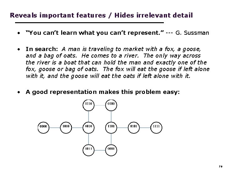
Reveals important features / Hides irrelevant detail • “You can’t learn what you can’t represent. ” --- G. Sussman • In search: A man is traveling to market with a fox, a goose, and a bag of oats. He comes to a river. The only way across the river is a boat that can hold the man and exactly one of the fox, goose or bag of oats. The fox will eat the goose if left alone with it, and the goose will eat the oats if left alone with it. • A good representation makes this problem easy: 1110 0010 1111 0001 0101 78

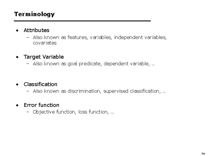
Terminology • Attributes – Also known as features, variables, independent variables, covariates • Target Variable – Also known as goal predicate, dependent variable, … • Classification – Also known as discrimination, supervised classification, … • Error function – Objective function, loss function, … 79

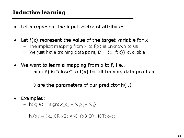
Inductive learning • Let x represent the input vector of attributes • Let f(x) represent the value of the target variable for x – The implicit mapping from x to f(x) is unknown to us – We just have training data pairs, D = {x, f(x)} available • We want to learn a mapping from x to f, i. e. , h(x; ) is “close” to f(x) for all training data points x are the parameters of our predictor h(. . ) • Examples: – h(x; ) = sign(w 1 x 1 + w 2 x 2+ w 3) – hk(x) = (x 1 OR x 2) AND (x 3 OR NOT(x 4)) 80

Empirical Error Functions • Empirical error function: E(h) = x distance[h(x; ) , f] e. g. , distance = squared error if h and f are real-valued (regression) distance = delta-function if h and f are categorical (classification) Sum is over all training pairs in the training data D In learning, we get to choose 1. what class of functions h(. . ) that we want to learn – potentially a huge space! (“hypothesis space”) 2. what error function/distance to use - should be chosen to reflect real “loss” in problem - but often chosen for mathematical/algorithmic convenience 81

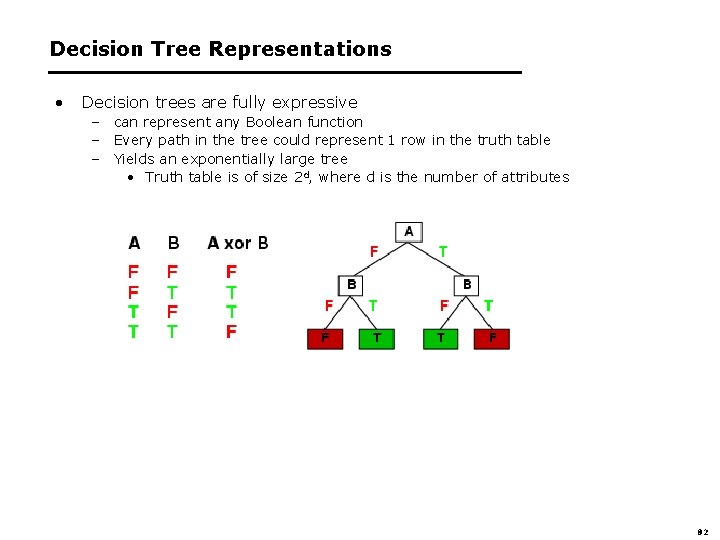
Decision Tree Representations • Decision trees are fully expressive – can represent any Boolean function – Every path in the tree could represent 1 row in the truth table – Yields an exponentially large tree • Truth table is of size 2 d, where d is the number of attributes 82

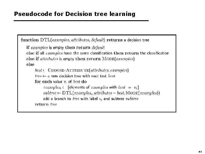
Pseudocode for Decision tree learning 83

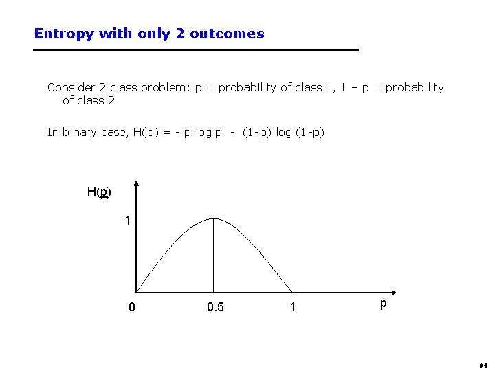
Entropy with only 2 outcomes Consider 2 class problem: p = probability of class 1, 1 – p = probability of class 2 In binary case, H(p) = - p log p - (1 -p) log (1 -p) H(p) 1 0 0. 5 1 p 84

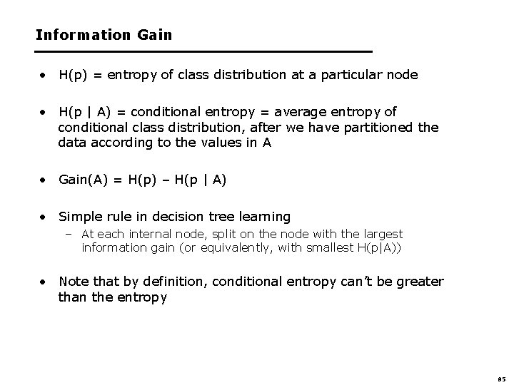
Information Gain • H(p) = entropy of class distribution at a particular node • H(p | A) = conditional entropy = average entropy of conditional class distribution, after we have partitioned the data according to the values in A • Gain(A) = H(p) – H(p | A) • Simple rule in decision tree learning – At each internal node, split on the node with the largest information gain (or equivalently, with smallest H(p|A)) • Note that by definition, conditional entropy can’t be greater than the entropy 85

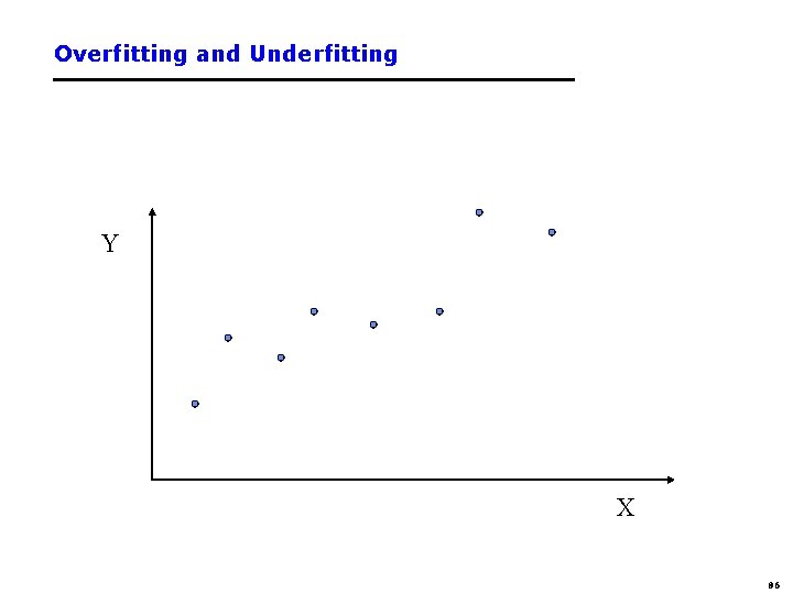
Overfitting and Underfitting Y X 86

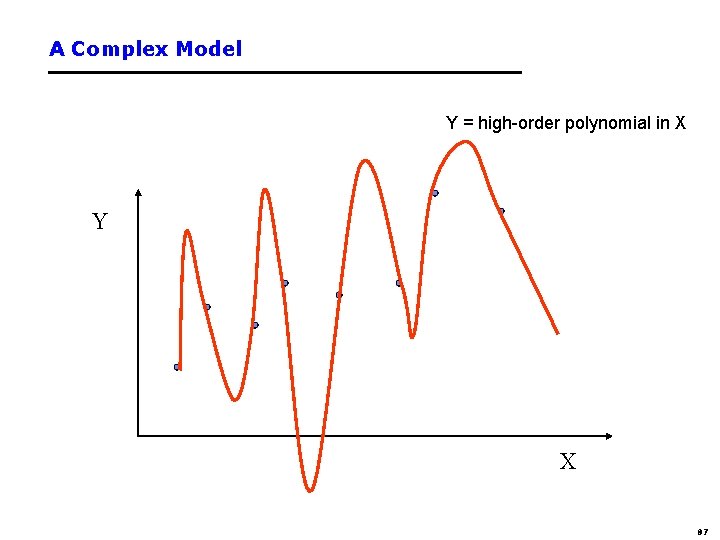
A Complex Model Y = high-order polynomial in X Y X 87

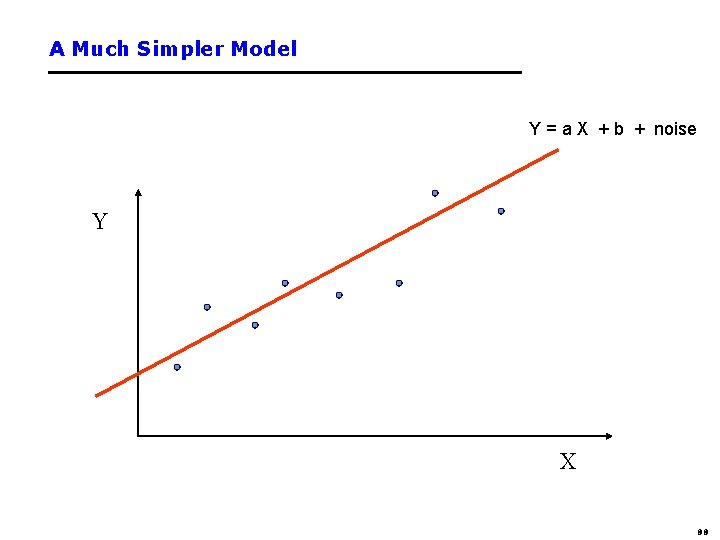
A Much Simpler Model Y = a X + b + noise Y X 88

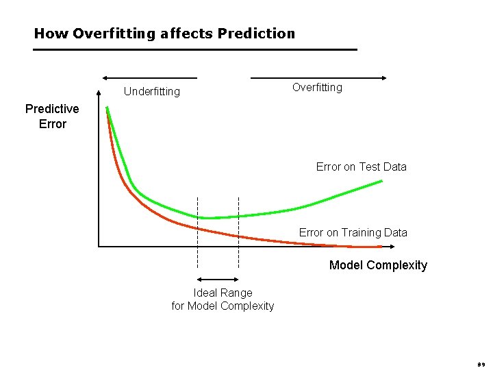
How Overfitting affects Prediction Underfitting Overfitting Predictive Error on Test Data Error on Training Data Model Complexity Ideal Range for Model Complexity 89

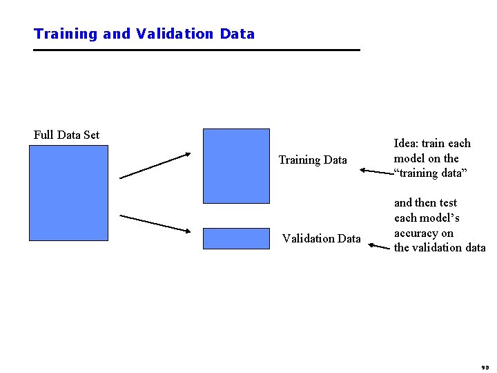
Training and Validation Data Full Data Set Training Data Validation Data Idea: train each model on the “training data” and then test each model’s accuracy on the validation data 90

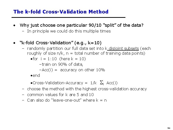
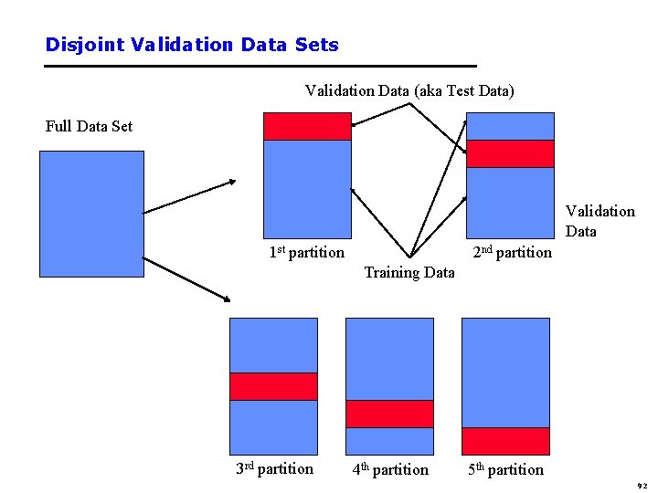
The k-fold Cross-Validation Method • Why just choose one particular 90/10 “split” of the data? – In principle we could do this multiple times • “k-fold Cross-Validation” (e. g. , k=10) – randomly partition our full data set into k disjoint subsets (each roughly of size n/k, n = total number of training data points) • for i = 1: 10 (here k = 10) –train on 90% of data, –Acc(i) = accuracy on other 10% • end • Cross-Validation-Accuracy = 1/k i Acc(i) – choose the method with the highest cross-validation accuracy – common values for k are 5 and 10 – Can also do “leave-one-out” where k = n 91

Disjoint Validation Data Sets Validation Data (aka Test Data) Full Data Set Validation Data 1 st partition 2 nd partition Training Data 3 rd partition 4 th partition 5 th partition 92

CS-271 P Final Review • Propositional Logic • (7. 1 -7. 5) • First-Order Logic, Knowledge Representation • (8. 1 -8. 5, 9. 1 -9. 2) • Constraint Satisfaction Problems • (6. 1 -6. 4, except 6. 3) • Machine Learning • (18. 1 -18. 4) • Questions on any topic • Pre-mid-term material if time and class interest • Please review your quizzes, mid-term, & old tests • At least one question from a prior quiz or test will appear on the Final Exam (and all other tests) 114