Chapter 10 Algorithm Efficiency and Sorting 2006 Pearson

Chapter 10 Algorithm Efficiency and Sorting © 2006 Pearson Addison-Wesley. All rights reserved 1

Measuring the Efficiency of Algorithms • Analysis of algorithms – Provides tools for contrasting the efficiency of different methods of solution • A comparison of algorithms – Should focus of significant differences in efficiency – Should not consider reductions in computing costs due to clever coding tricks © 2006 Pearson Addison-Wesley. All rights reserved 2

Measuring the Efficiency of Algorithms • Three difficulties with comparing programs instead of algorithms – How are the algorithms coded? – What computer should you use? – What data should the programs use? • Algorithm analysis should be independent of – Specific implementations – Computers – Data © 2006 Pearson Addison-Wesley. All rights reserved 3

The Execution Time of Algorithms • Counting an algorithm's operations is a way to access its efficiency – An algorithm’s execution time is related to the number of operations it requires – Examples • Traversal of a linked list • The Towers of Hanoi • Nested Loops © 2006 Pearson Addison-Wesley. All rights reserved 4

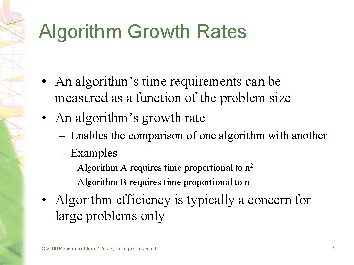
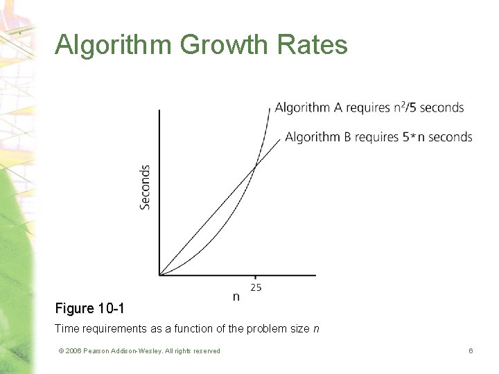
Algorithm Growth Rates • An algorithm’s time requirements can be measured as a function of the problem size • An algorithm’s growth rate – Enables the comparison of one algorithm with another – Examples Algorithm A requires time proportional to n 2 Algorithm B requires time proportional to n • Algorithm efficiency is typically a concern for large problems only © 2006 Pearson Addison-Wesley. All rights reserved 5

Algorithm Growth Rates Figure 10 -1 Time requirements as a function of the problem size n © 2006 Pearson Addison-Wesley. All rights reserved 6

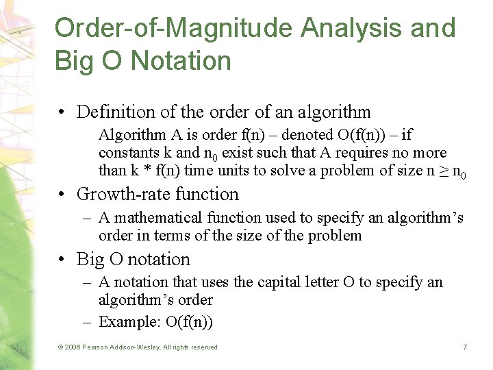
Order-of-Magnitude Analysis and Big O Notation • Definition of the order of an algorithm A is order f(n) – denoted O(f(n)) – if constants k and n 0 exist such that A requires no more than k * f(n) time units to solve a problem of size n ≥ n 0 • Growth-rate function – A mathematical function used to specify an algorithm’s order in terms of the size of the problem • Big O notation – A notation that uses the capital letter O to specify an algorithm’s order – Example: O(f(n)) © 2006 Pearson Addison-Wesley. All rights reserved 7

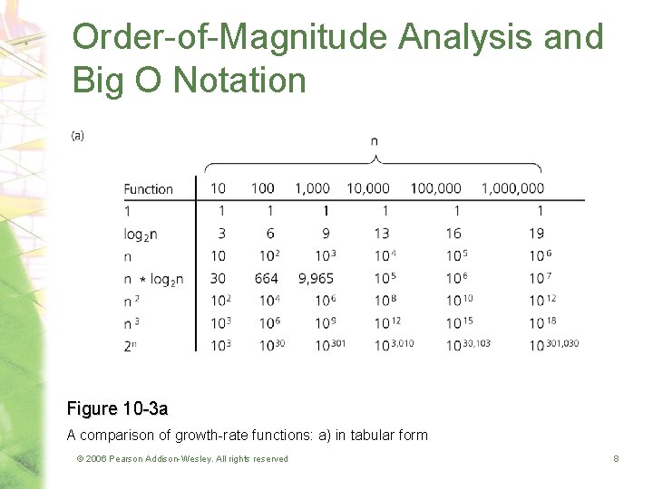
Order-of-Magnitude Analysis and Big O Notation Figure 10 -3 a A comparison of growth-rate functions: a) in tabular form © 2006 Pearson Addison-Wesley. All rights reserved 8

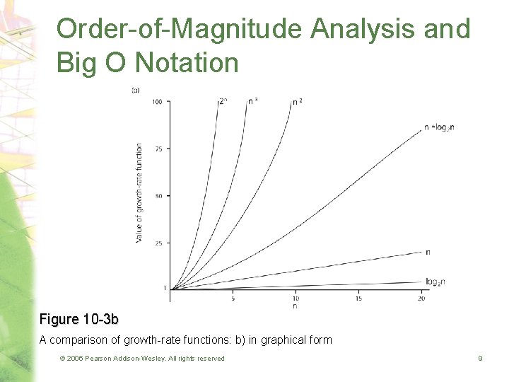
Order-of-Magnitude Analysis and Big O Notation Figure 10 -3 b A comparison of growth-rate functions: b) in graphical form © 2006 Pearson Addison-Wesley. All rights reserved 9

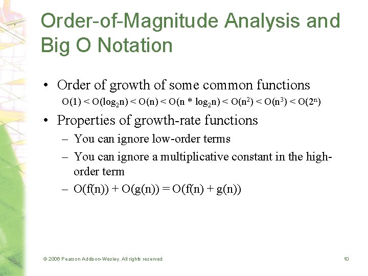
Order-of-Magnitude Analysis and Big O Notation • Order of growth of some common functions O(1) < O(log 2 n) < O(n * log 2 n) < O(n 2) < O(n 3) < O(2 n) • Properties of growth-rate functions – You can ignore low-order terms – You can ignore a multiplicative constant in the highorder term – O(f(n)) + O(g(n)) = O(f(n) + g(n)) © 2006 Pearson Addison-Wesley. All rights reserved 10

Order-of-Magnitude Analysis and Big O Notation • Worst-case and average-case analyses – An algorithm can require different times to solve different problems of the same size • Worst-case analysis – A determination of the maximum amount of time that an algorithm requires to solve problems of size n • Average-case analysis – A determination of the average amount of time that an algorithm requires to solve problems of size n © 2006 Pearson Addison-Wesley. All rights reserved 11

Keeping Your Perspective • Throughout the course of an analysis, keep in mind that you are interested only in significant differences in efficiency • When choosing an ADT’s implementation, consider how frequently particular ADT operations occur in a given application • Some seldom-used but critical operations must be efficient © 2006 Pearson Addison-Wesley. All rights reserved 12

Keeping Your Perspective • If the problem size is always small, you can probably ignore an algorithm’s efficiency • Weigh the trade-offs between an algorithm’s time requirements and its memory requirements • Compare algorithms for both style and efficiency • Order-of-magnitude analysis focuses on large problems © 2006 Pearson Addison-Wesley. All rights reserved 13

The Efficiency of Searching Algorithms • Sequential search – Strategy • Look at each item in the data collection in turn, beginning with the first one • Stop when – You find the desired item – You reach the end of the data collection © 2006 Pearson Addison-Wesley. All rights reserved 14

The Efficiency of Searching Algorithms • Sequential search – Efficiency • Worst case: O(n) • Average case: O(n) • Best case: O(1) © 2006 Pearson Addison-Wesley. All rights reserved 15

The Efficiency of Searching Algorithms • Binary search – Strategy • To search a sorted array for a particular item – Repeatedly divide the array in half – Determine which half the item must be in, if it is indeed present, and discard the other half – Efficiency • Worst case: O(log 2 n) • For large arrays, the binary search has an enormous advantage over a sequential search © 2006 Pearson Addison-Wesley. All rights reserved 16

Sorting Algorithms and Their Efficiency • Sorting – A process that organizes a collection of data into either ascending or descending order • Categories of sorting algorithms – An internal sort • Requires that the collection of data fit entirely in the computer’s main memory – An external sort • The collection of data will not fit in the computer’s main memory all at once but must reside in secondary storage © 2006 Pearson Addison-Wesley. All rights reserved 17

Sorting Algorithms and Their Efficiency • Data items to be sorted can be – Integers – Character strings – Objects • Sort key – The part of a record that determines the sorted order of the entire record within a collection of records © 2006 Pearson Addison-Wesley. All rights reserved 18

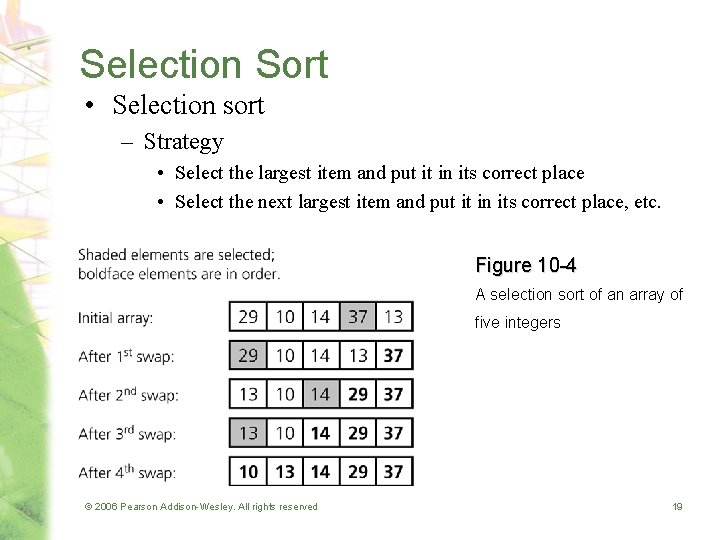
Selection Sort • Selection sort – Strategy • Select the largest item and put it in its correct place • Select the next largest item and put it in its correct place, etc. Figure 10 -4 A selection sort of an array of five integers © 2006 Pearson Addison-Wesley. All rights reserved 19

Selection Sort • Analysis – Selection sort is O(n 2) • Advantage of selection sort – It does not depend on the initial arrangement of the data • Disadvantage of selection sort – It is only appropriate for small n © 2006 Pearson Addison-Wesley. All rights reserved 20

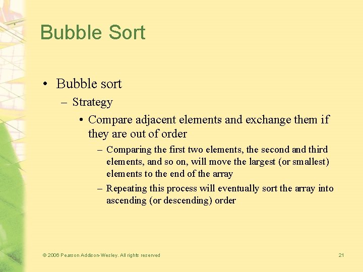
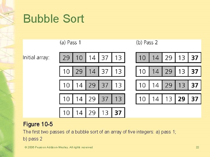
Bubble Sort • Bubble sort – Strategy • Compare adjacent elements and exchange them if they are out of order – Comparing the first two elements, the second and third elements, and so on, will move the largest (or smallest) elements to the end of the array – Repeating this process will eventually sort the array into ascending (or descending) order © 2006 Pearson Addison-Wesley. All rights reserved 21

Bubble Sort Figure 10 -5 The first two passes of a bubble sort of an array of five integers: a) pass 1; b) pass 2 © 2006 Pearson Addison-Wesley. All rights reserved 22

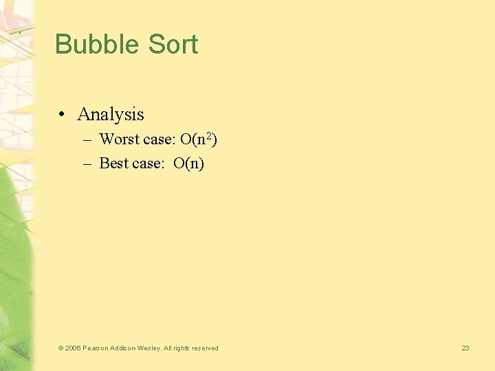
Bubble Sort • Analysis – Worst case: O(n 2) – Best case: O(n) © 2006 Pearson Addison-Wesley. All rights reserved 23

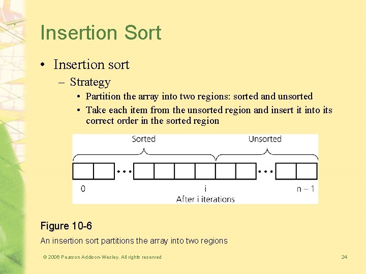
Insertion Sort • Insertion sort – Strategy • Partition the array into two regions: sorted and unsorted • Take each item from the unsorted region and insert it into its correct order in the sorted region Figure 10 -6 An insertion sort partitions the array into two regions © 2006 Pearson Addison-Wesley. All rights reserved 24

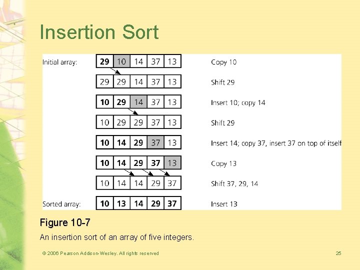
Insertion Sort Figure 10 -7 An insertion sort of an array of five integers. © 2006 Pearson Addison-Wesley. All rights reserved 25

Insertion Sort • Analysis – Worst case: O(n 2) – For small arrays • Insertion sort is appropriate due to its simplicity – For large arrays • Insertion sort is prohibitively inefficient © 2006 Pearson Addison-Wesley. All rights reserved 26

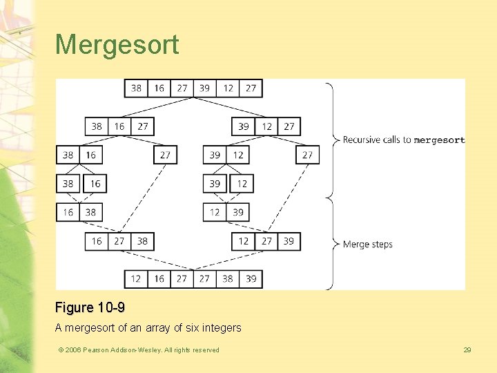
Mergesort • Important divide-and-conquer sorting algorithms – Mergesort – Quicksort • Mergesort – A recursive sorting algorithm – Gives the same performance, regardless of the initial order of the array items – Strategy • Divide an array into halves • Sort each half • Merge the sorted halves into one sorted array © 2006 Pearson Addison-Wesley. All rights reserved 27

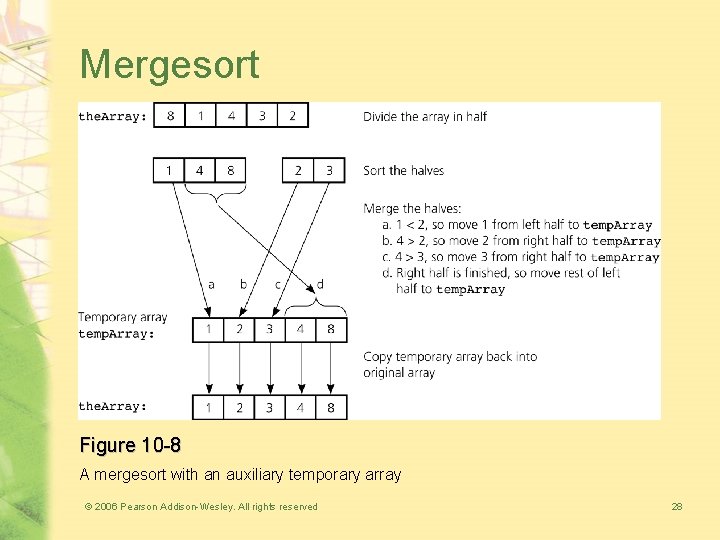
Mergesort Figure 10 -8 A mergesort with an auxiliary temporary array © 2006 Pearson Addison-Wesley. All rights reserved 28

Mergesort Figure 10 -9 A mergesort of an array of six integers © 2006 Pearson Addison-Wesley. All rights reserved 29

Mergesort • Analysis – Worst case: O(n * log 2 n) – Average case: O(n * log 2 n) – Advantage • It is an extremely efficient algorithm with respect to time – Drawback • It requires a second array as large as the original array © 2006 Pearson Addison-Wesley. All rights reserved 30

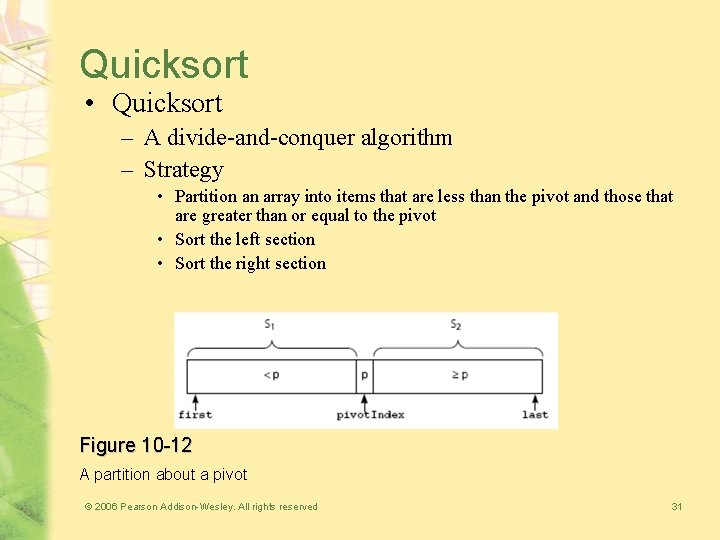
Quicksort • Quicksort – A divide-and-conquer algorithm – Strategy • Partition an array into items that are less than the pivot and those that are greater than or equal to the pivot • Sort the left section • Sort the right section Figure 10 -12 A partition about a pivot © 2006 Pearson Addison-Wesley. All rights reserved 31

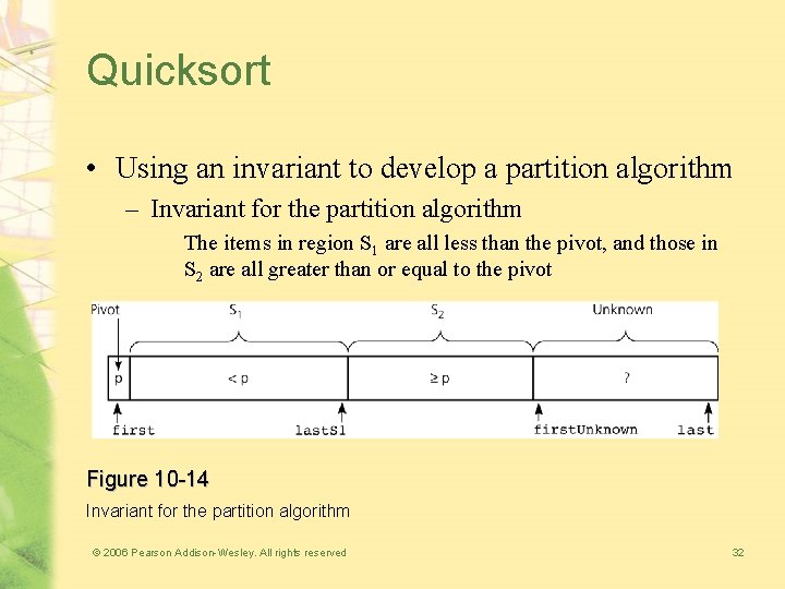
Quicksort • Using an invariant to develop a partition algorithm – Invariant for the partition algorithm The items in region S 1 are all less than the pivot, and those in S 2 are all greater than or equal to the pivot Figure 10 -14 Invariant for the partition algorithm © 2006 Pearson Addison-Wesley. All rights reserved 32

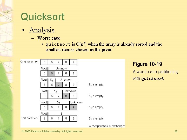
Quicksort • Analysis – Worst case • quicksort is O(n 2) when the array is already sorted and the smallest item is chosen as the pivot Figure 10 -19 A worst-case partitioning with quicksort © 2006 Pearson Addison-Wesley. All rights reserved 33

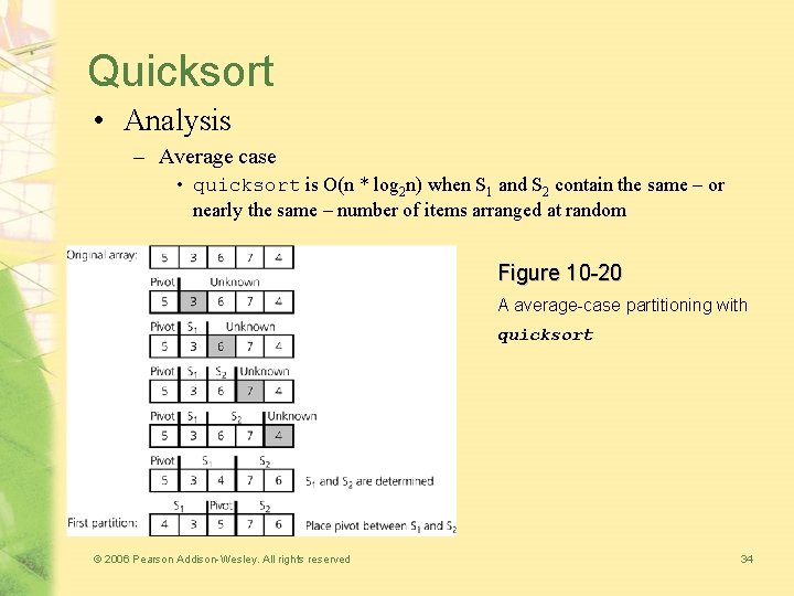
Quicksort • Analysis – Average case • quicksort is O(n * log 2 n) when S 1 and S 2 contain the same – or nearly the same – number of items arranged at random Figure 10 -20 A average-case partitioning with quicksort © 2006 Pearson Addison-Wesley. All rights reserved 34

Quicksort • Analysis – quicksort is usually extremely fast in practice – Even if the worst case occurs, quicksort’s performance is acceptable for moderately large arrays © 2006 Pearson Addison-Wesley. All rights reserved 35

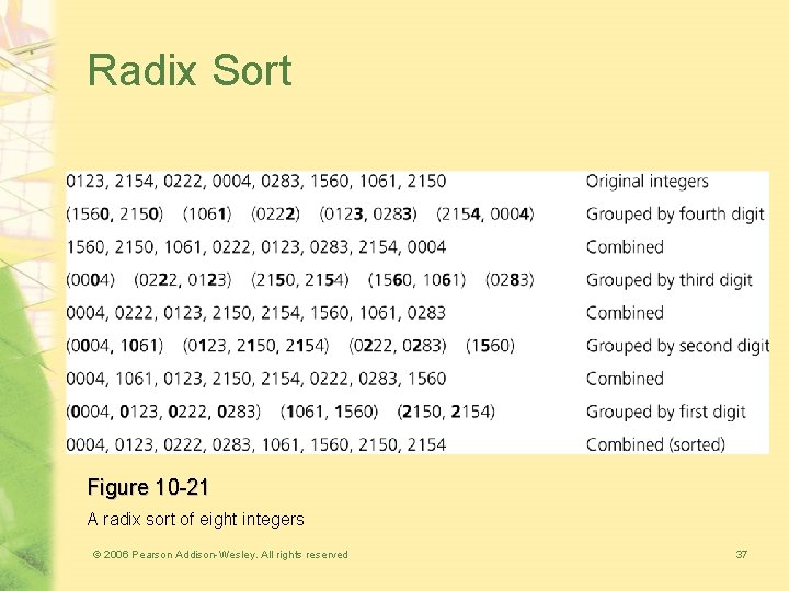
Radix Sort • Radix sort – Treats each data element as a character string – Strategy • Repeatedly organize the data into groups according to the ith character in each element • Analysis – Radix sort is O(n) © 2006 Pearson Addison-Wesley. All rights reserved 36

Radix Sort Figure 10 -21 A radix sort of eight integers © 2006 Pearson Addison-Wesley. All rights reserved 37

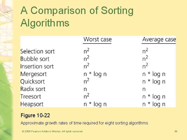
A Comparison of Sorting Algorithms Figure 10 -22 Approximate growth rates of time required for eight sorting algorithms © 2006 Pearson Addison-Wesley. All rights reserved 38

Summary • Order-of-magnitude analysis and Big O notation measure an algorithm’s time requirement as a function of the problem size by using a growthrate function • To compare the inherit efficiency of algorithms – Examine their growth-rate functions when the problems are large – Consider only significant differences in growth-rate functions © 2006 Pearson Addison-Wesley. All rights reserved 39

Summary • Worst-case and average-case analyses – Worst-case analysis considers the maximum amount of work an algorithm requires on a problem of a given size – Average-case analysis considers the expected amount of work an algorithm requires on a problem of a given size • Order-of-magnitude analysis can be used to choose an implementation for an abstract data type • Selection sort, bubble sort, and insertion sort are all O(n 2) algorithms • Quicksort and mergesort are two very efficient sorting algorithms © 2006 Pearson Addison-Wesley. All rights reserved 40