Artificiel Neural Networks 2 Morten Nielsen Department of

Artificiel Neural Networks 2 Morten Nielsen Department of Health Technology, DTU

Outline • Optimization procedures – Gradient decent (this you already know) • Network training – – – back propagation cross-validation Over-fitting Examples Deeplearning

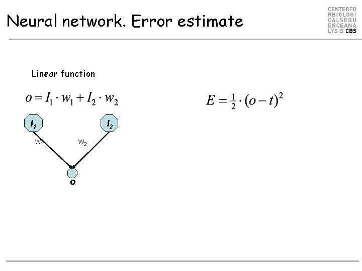
Neural network. Error estimate Linear function I 2 I 1 w 2 o

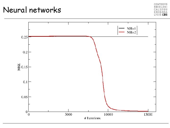
Neural networks

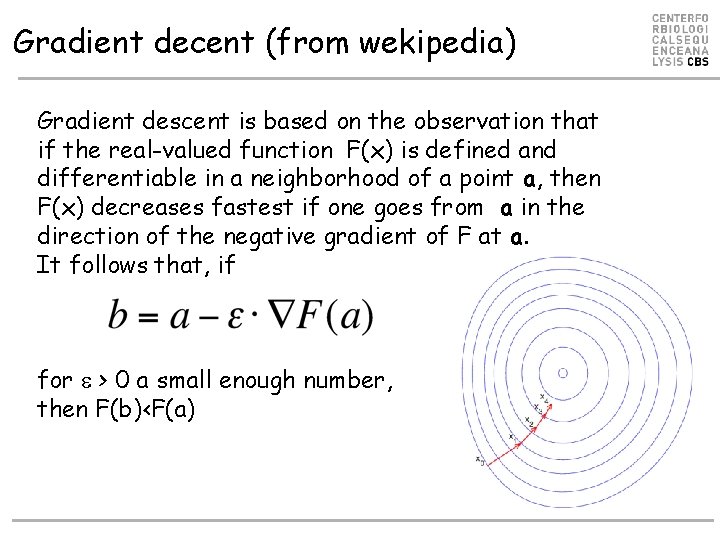
Gradient decent (from wekipedia) Gradient descent is based on the observation that if the real-valued function F(x) is defined and differentiable in a neighborhood of a point a, then F(x) decreases fastest if one goes from a in the direction of the negative gradient of F at a. It follows that, if for > 0 a small enough number, then F(b)<F(a)

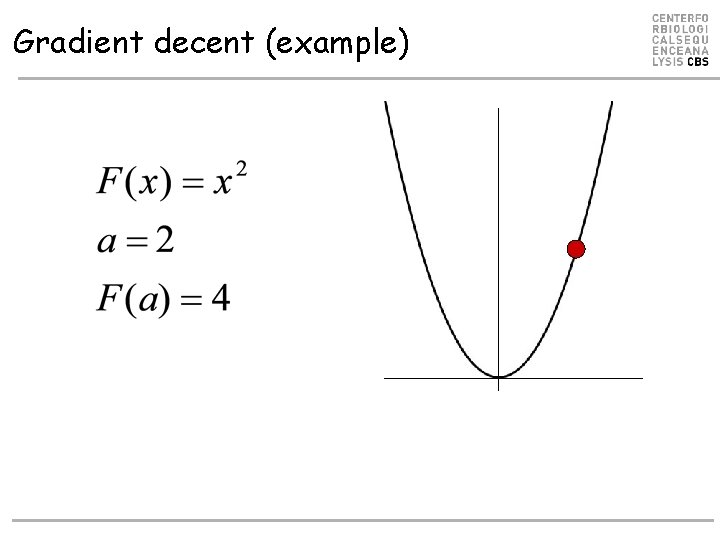
Gradient decent (example)

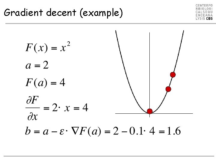
Gradient decent (example)

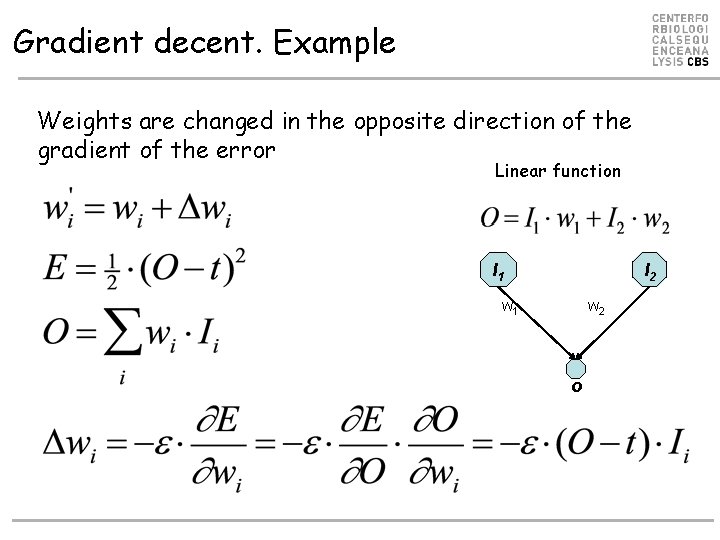
Gradient decent. Example Weights are changed in the opposite direction of the gradient of the error Linear function I 1 I 2 w 1 w 2 o

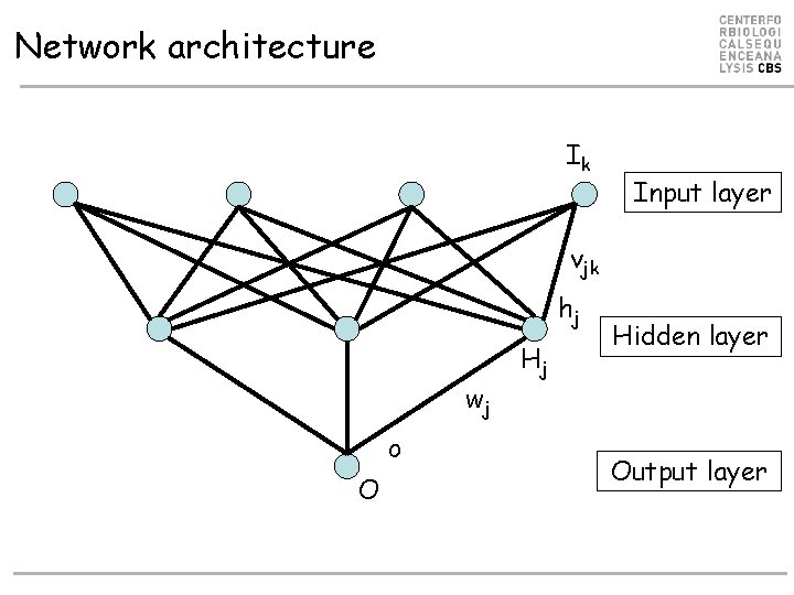
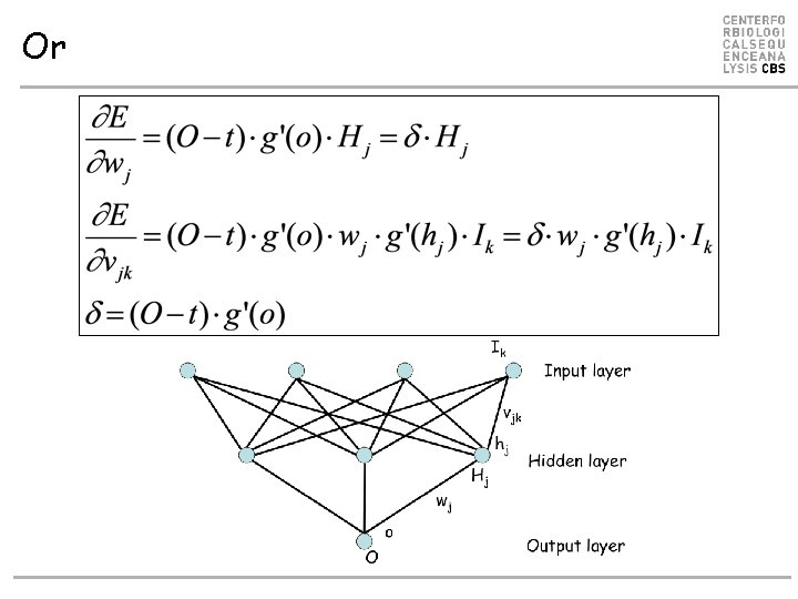
Network architecture Ik Input layer vjk hj wj o O Hj Hidden layer Output layer

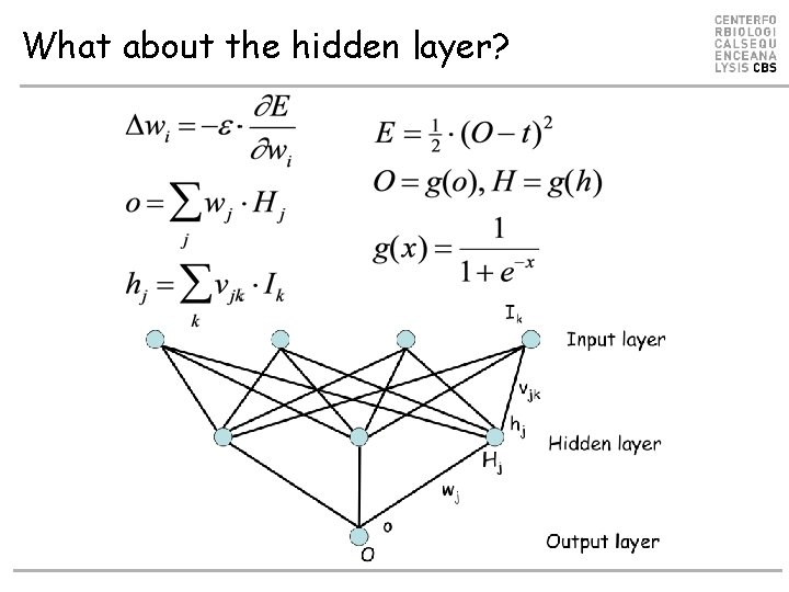
What about the hidden layer?

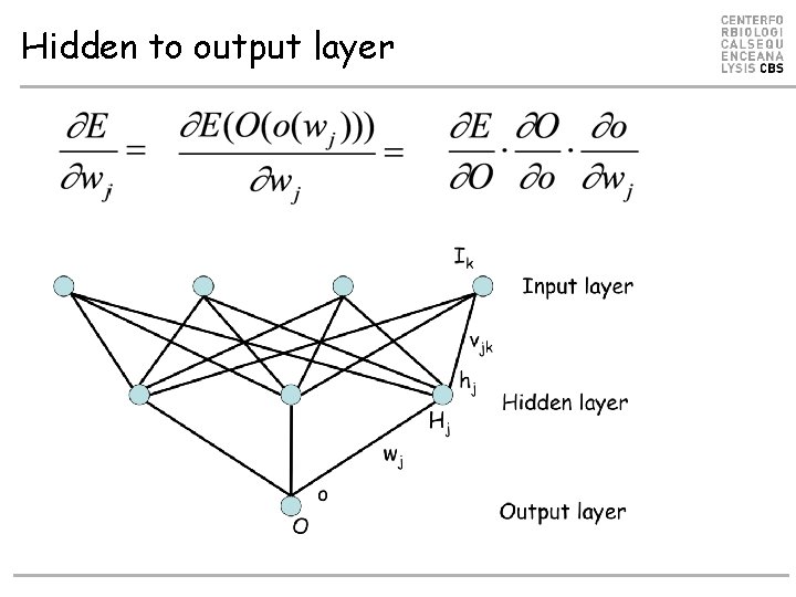
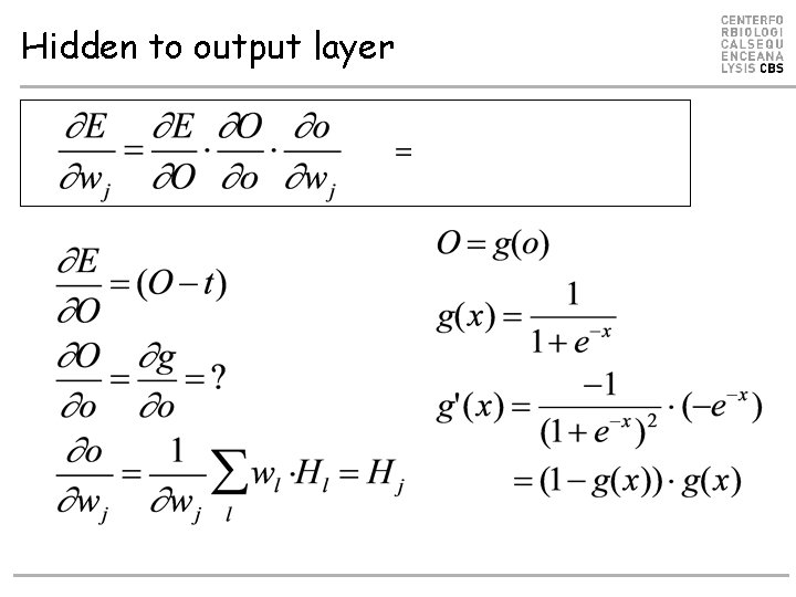
Hidden to output layer

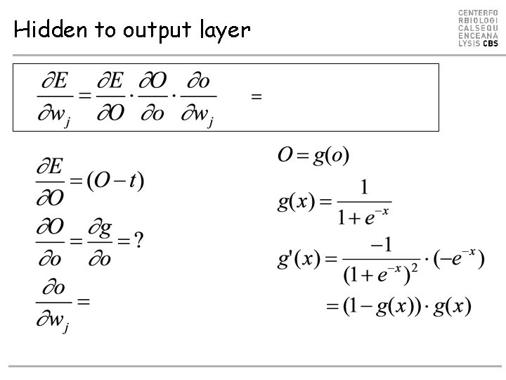
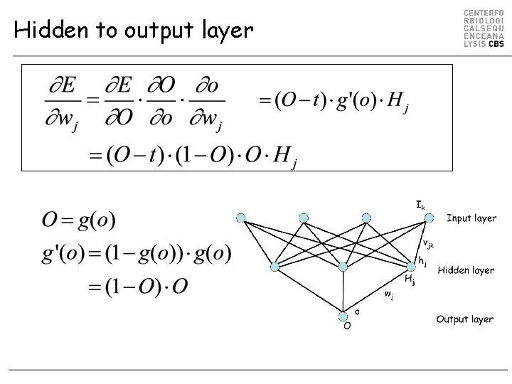
Hidden to output layer

Hidden to output layer

Hidden to output layer

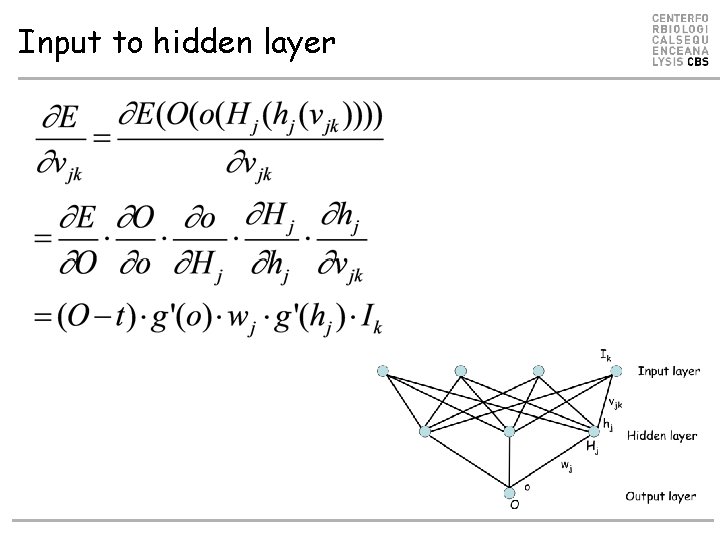
Input to hidden layer

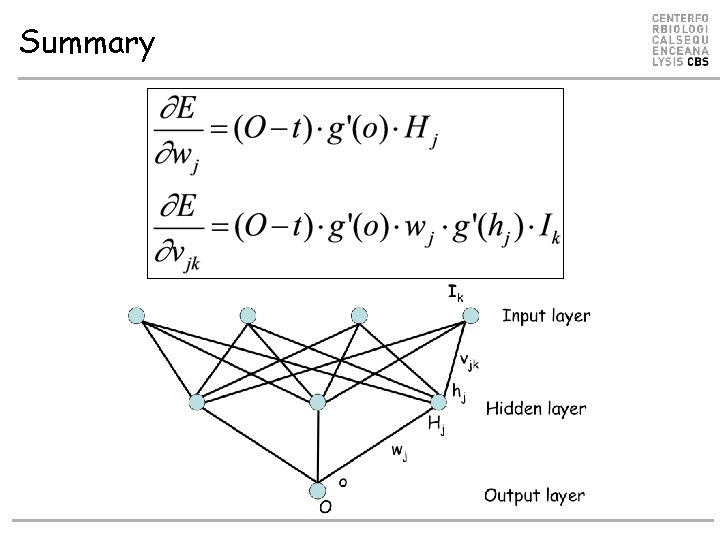
Summary

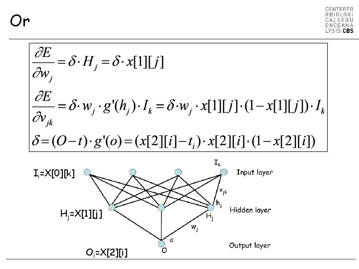
Or

Or Ii=X[0][k] Hj=X[1][j] Oi=X[2][i]

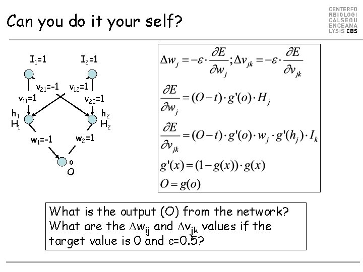
Can you do it your self? I 1=1 I 2=1 v 21=-1 v 11=1 v 12=1 v 22=1 h 1 H 1 w 2=1 w 1=-1 h 2 H 2 o O What is the output (O) from the network? What are the wij and vjk values if the target value is 0 and =0. 5?

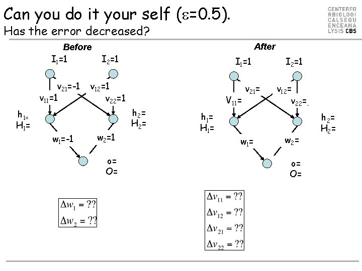
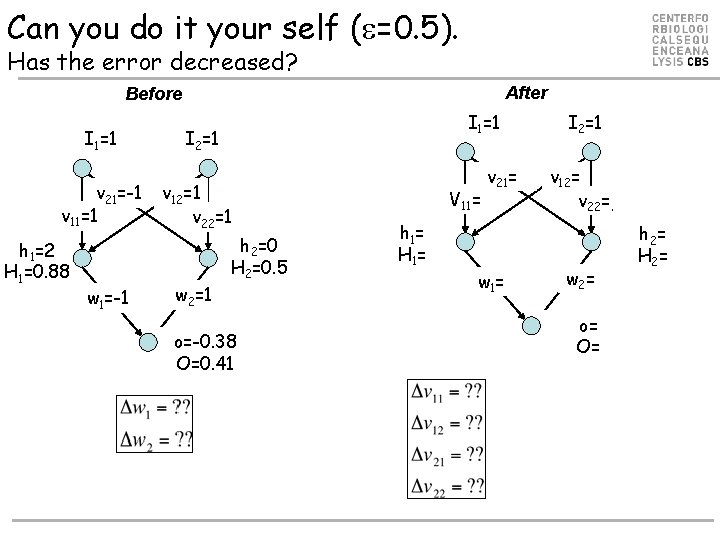
Can you do it your self ( =0. 5). Has the error decreased? Before I 1=1 v 21=-1 v 11=1 h 1= H 1 = w 1=-1 After I 2=1 I 1=1 v 12=1 v 22=1 w 2=1 o= O= h 2= H 2 = V 11= h 1 = H 1 = v 21= w 1 = I 2=1 v 12= v 22=. w 2 = o= O= h 2= H 2 =

Can you do it your self ( =0. 5). Has the error decreased? After Before I 1=1 v 21=-1 v 11=1 h 1=2 H 1=0. 88 w 1=-1 I 1=1 I 2=1 v 12=1 v 22=1 w 2=1 h 2=0 H 2=0. 5 o=-0. 38 O=0. 41 V 11= h 1 = H 1 = v 21= w 1 = I 2=1 v 12= v 22=. w 2 = o= O= h 2= H 2 =

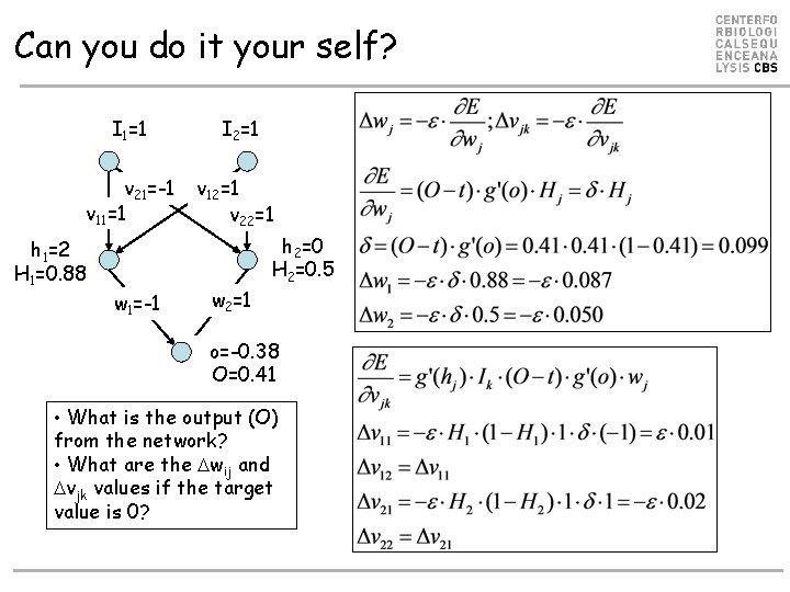
Can you do it your self? I 1=1 I 2=1 v 21=-1 v 11=1 v 12=1 v 22=1 h 1=2 H 1=0. 88 w 1=-1 w 2=1 h 2=0 H 2=0. 5 o=-0. 38 O=0. 41 • What is the output (O) from the network? • What are the wij and vjk values if the target value is 0?

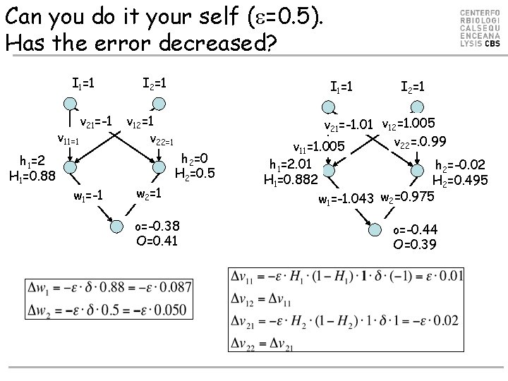
Can you do it your self ( =0. 5). Has the error decreased? I 1=1 v 11=1 h 1=2 H 1=0. 88 v 21=-1 w 1=-1 I 2=1 I 1=1 v 12=1 v 22=1 w 2=1 h 2=0 H 2=0. 5 o=-0. 38 O=0. 41 I 2=1 v 21=-1. 01 v 12=1. 005 v 22=. 0. 99 v 11=1. 005 h 1=2. 01 h 2=-0. 02 H 1=0. 882 H 2=0. 495 w 1=-1. 043 w 2=0. 975 o=-0. 44 O=0. 39

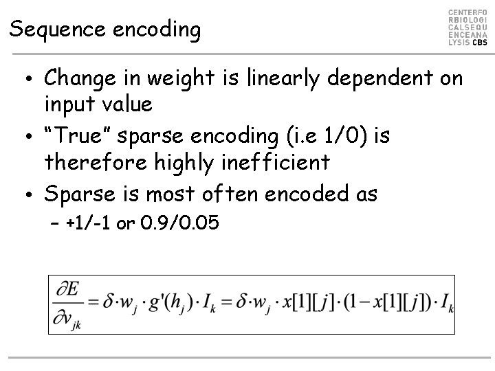
Sequence encoding • Change in weight is linearly dependent on input value • “True” sparse encoding (i. e 1/0) is therefore highly inefficient • Sparse is most often encoded as – +1/-1 or 0. 9/0. 05

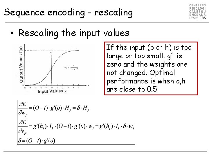
Sequence encoding - rescaling • Rescaling the input values If the input (o or h) is too large or too small, g´ is zero and the weights are not changed. Optimal performance is when o, h are close to 0. 5

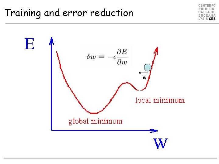
Training and error reduction

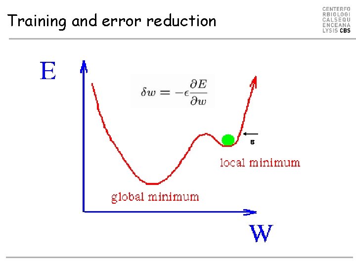
Training and error reduction

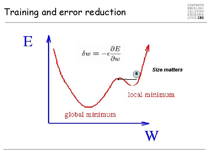
Training and error reduction Size matters

Demo • http: //playground. tensorflow. org/

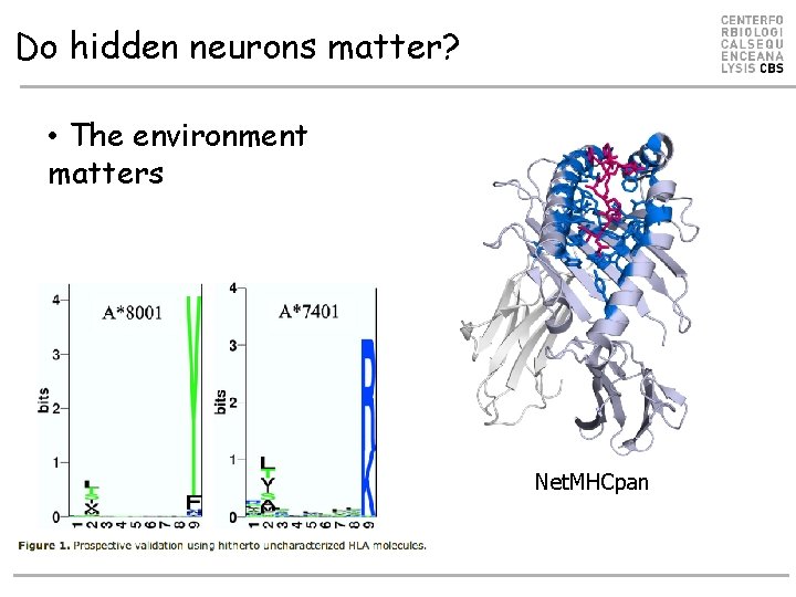
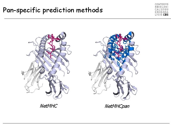
Do hidden neurons matter? • The environment matters Net. MHCpan

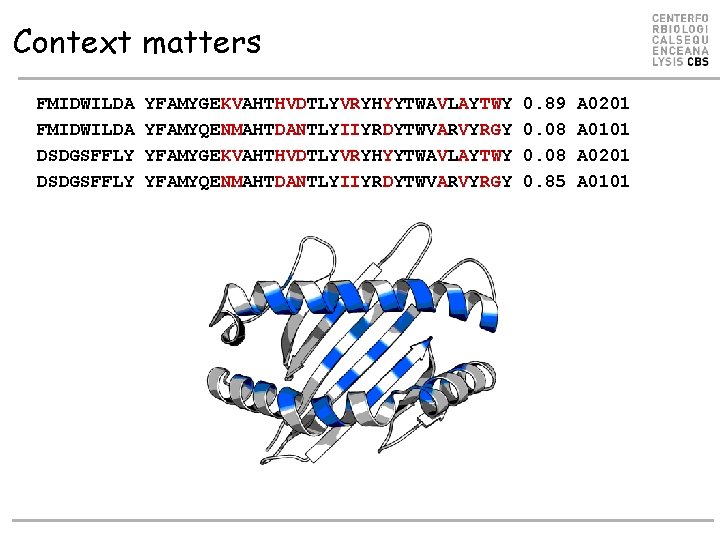
Context matters FMIDWILDA DSDGSFFLY YFAMYGEKVAHTHVDTLYVRYHYYTWAVLAYTWY YFAMYQENMAHTDANTLYIIYRDYTWVARVYRGY 0. 89 0. 08 0. 85 A 0201 A 0101

Summary • Gradient decent is used to determine the updates for the synapses in the neural network • Some relatively simple math defines the gradients – Networks without hidden layers can be solved on the back of an envelope (SMM exercise) – Hidden layers are a bit more complex, but still ok • Always train networks using a test set to stop training – Be careful when reporting predictive performance • Use “nested” cross-validation for small data sets • And hidden neurons do matter (sometimes)

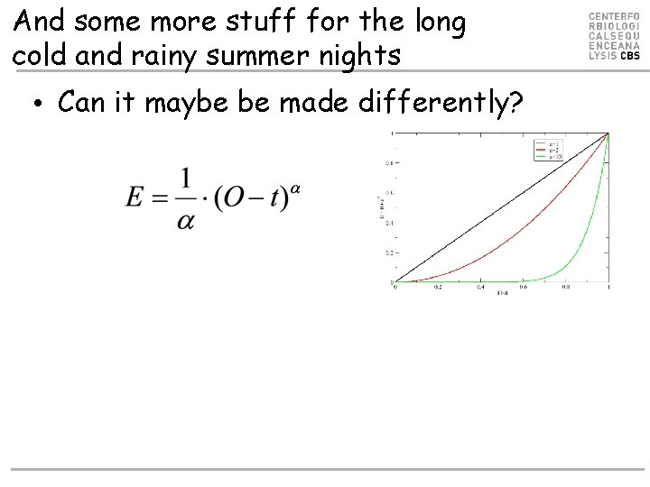
And some more stuff for the long cold and rainy summer nights • Can it maybe be made differently?

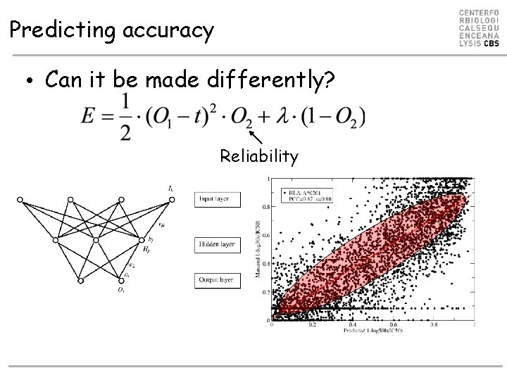
Predicting accuracy • Can it be made differently? Reliability

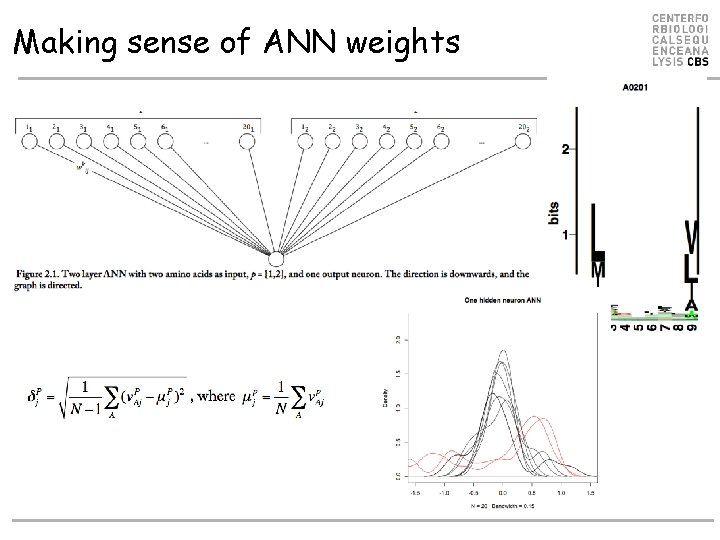
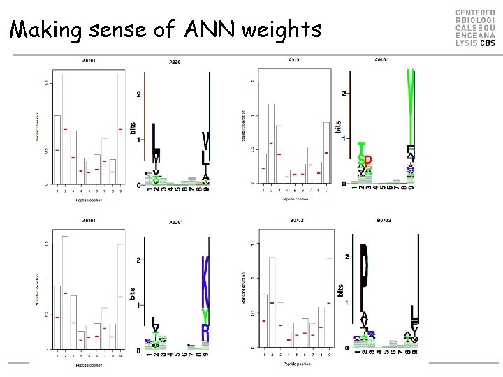
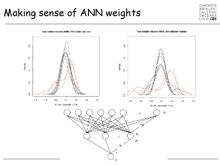
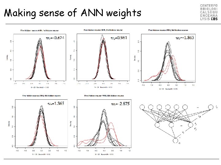
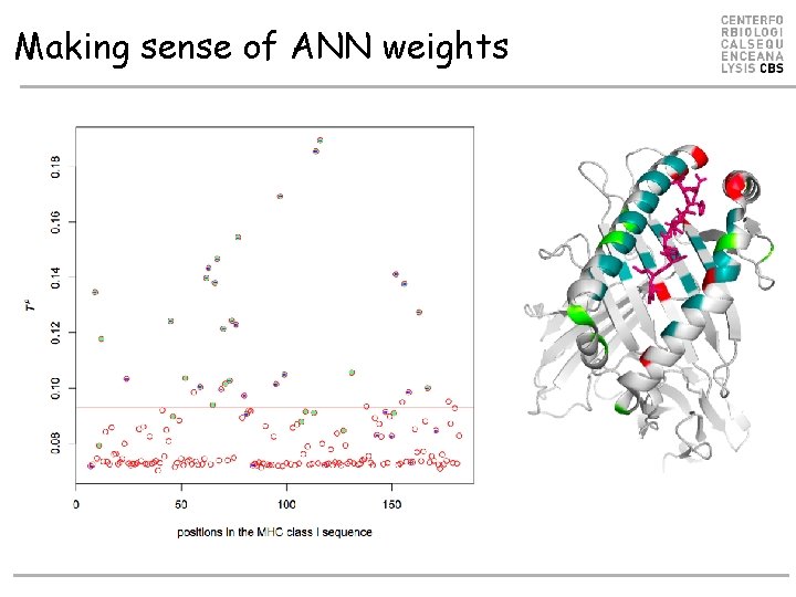
Making sense of ANN weights • Identification of position specific receptor ligand interactions by use of artificial neural network decomposition. An investigation of interactions in the MHC: peptide system Master thesis’ by Frederik Otzen Bagger and Piotr Chmura

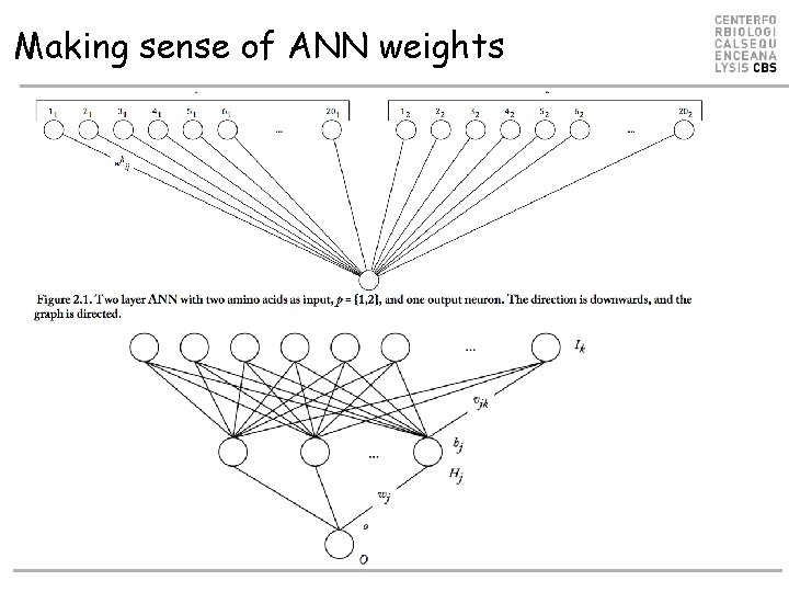
Making sense of ANN weights

Making sense of ANN weights

Making sense of ANN weights

Making sense of ANN weights

Making sense of ANN weights

Making sense of ANN weights

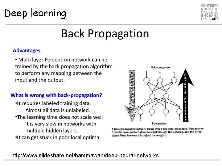
Deep learning http: //www. slideshare. net/hammawan/deep-neural-networks

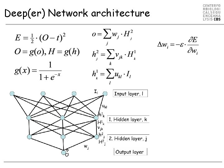
Deep(er) Network architecture

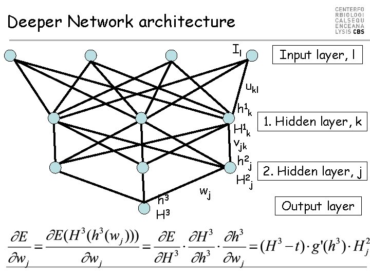
Deeper Network architecture Il Input layer, l ukl h 1 k H 1 k 1. Hidden layer, k vjk h 2 j h 3 H 3 wj H 2 j 2. Hidden layer, j Output layer

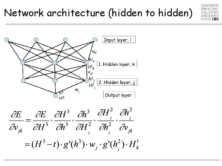
Network architecture (hidden to hidden)

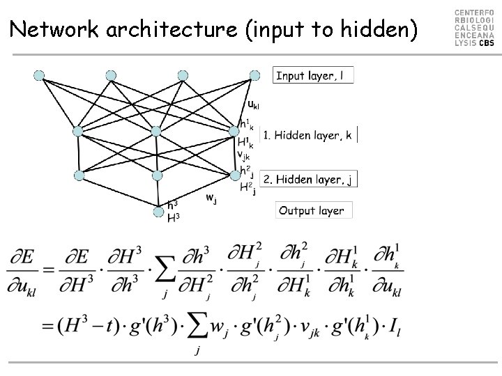
Network architecture (input to hidden)

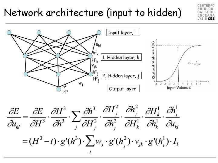
Network architecture (input to hidden)

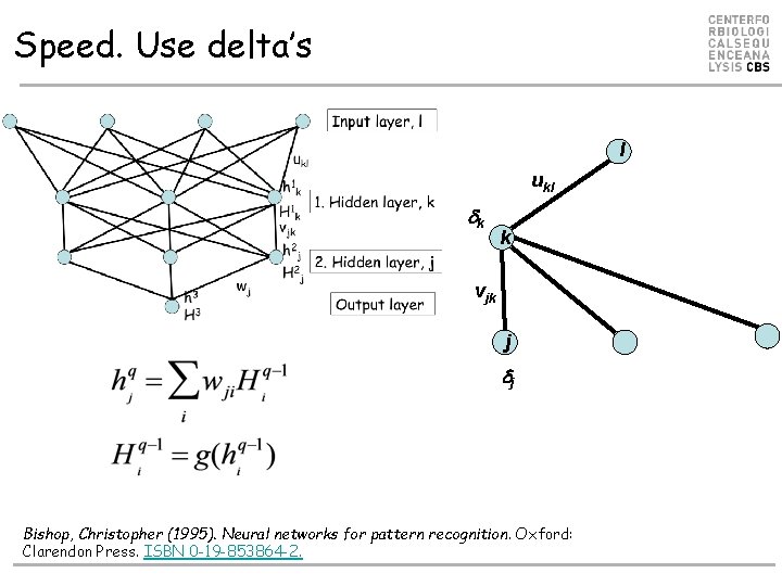
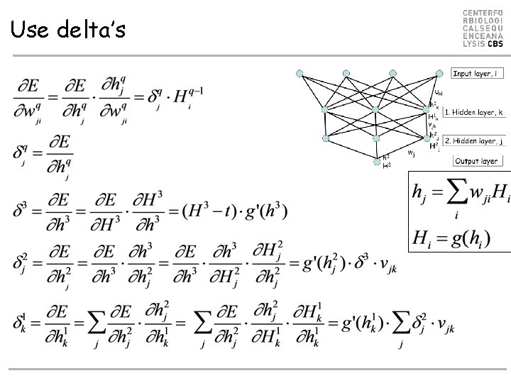
Speed. Use delta’s l ukl dk k vjk j dj Bishop, Christopher (1995). Neural networks for pattern recognition. Oxford: Clarendon Press. ISBN 0 -19 -853864 -2.

Use delta’s

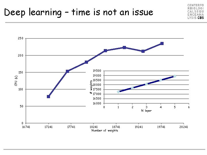
Deep learning – time is not an issue 250 200 19500 150 CPU (u) 19000 # weights 18500 18000 17500 17000 16500 16000 50 0 16741 17241 17741 0 1 18241 18741 Number of weights 2 3 N layer 19241 4 19741 5 6 20241

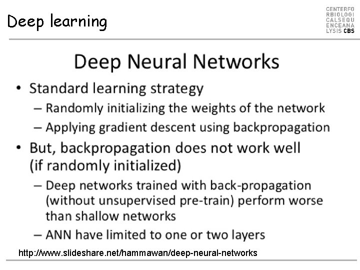
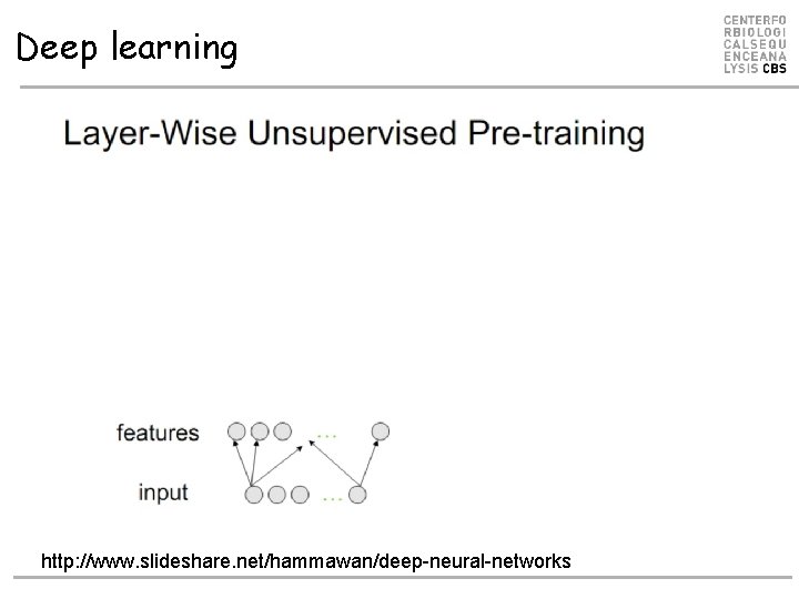
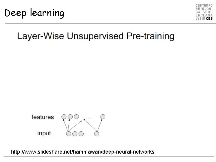
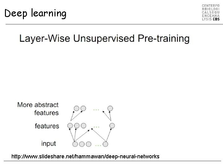
Deep learning http: //www. slideshare. net/hammawan/deep-neural-networks

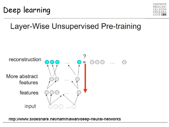
Deep learning http: //www. slideshare. net/hammawan/deep-neural-networks

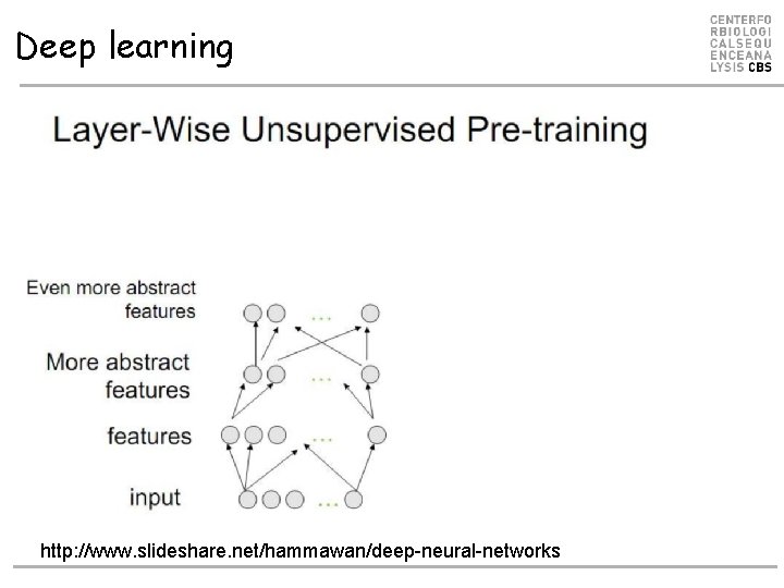
Deep learning http: //www. slideshare. net/hammawan/deep-neural-networks

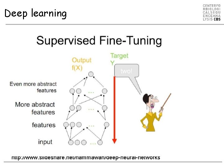
Deep learning http: //www. slideshare. net/hammawan/deep-neural-networks

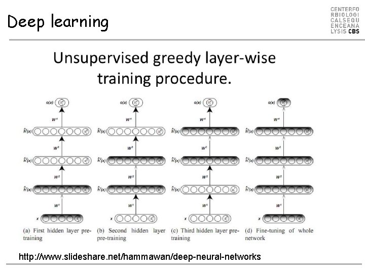
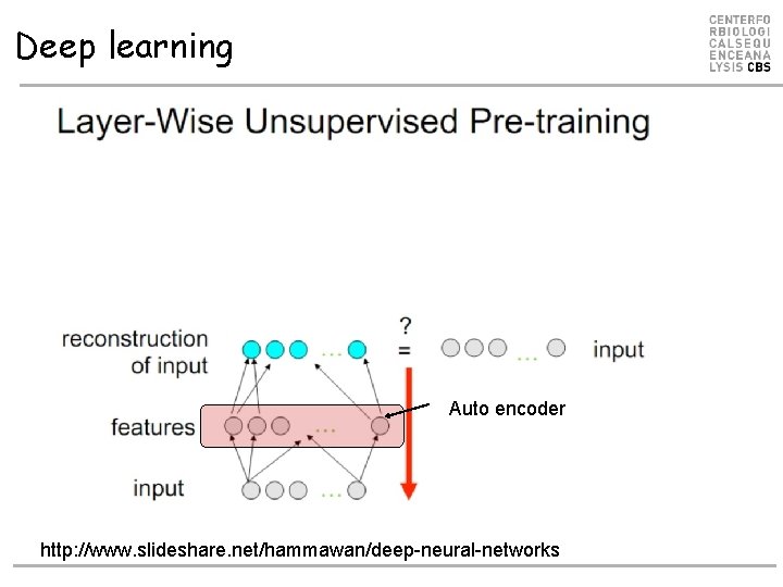
Deep learning Auto encoder http: //www. slideshare. net/hammawan/deep-neural-networks

Deep learning http: //www. slideshare. net/hammawan/deep-neural-networks

Deep learning http: //www. slideshare. net/hammawan/deep-neural-networks

Deep learning http: //www. slideshare. net/hammawan/deep-neural-networks

Deep learning http: //www. slideshare. net/hammawan/deep-neural-networks

Deep learning http: //www. slideshare. net/hammawan/deep-neural-networks

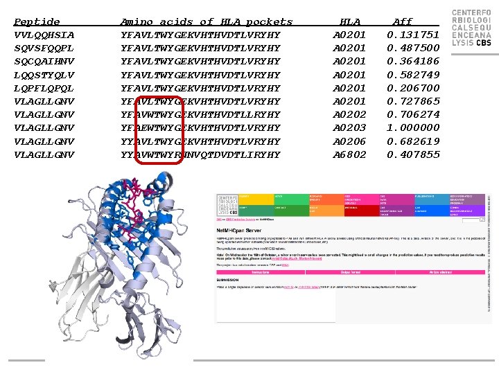
Pan-specific prediction methods Net. MHCpan

Example Peptide VVLQQHSIA SQVSFQQPL SQCQAIHNV LQQSTYQLV LQPFLQPQL VLAGLLGNV VLAGLLGNV Amino acids of HLA pockets YFAVLTWYGEKVHTHVDTLVRYHY YFAVLTWYGEKVHTHVDTLVRYHY YFAVWTWYGEKVHTHVDTLLRYHY YFAEWTWYGEKVHTHVDTLVRYHY YYAVLTWYGEKVHTHVDTLVRYHY YYAVWTWYRNNVQTDVDTLIRYHY HLA A 0201 A 0201 A 0202 A 0203 A 0206 A 6802 Aff 0. 131751 0. 487500 0. 364186 0. 582749 0. 206700 0. 727865 0. 706274 1. 000000 0. 682619 0. 407855

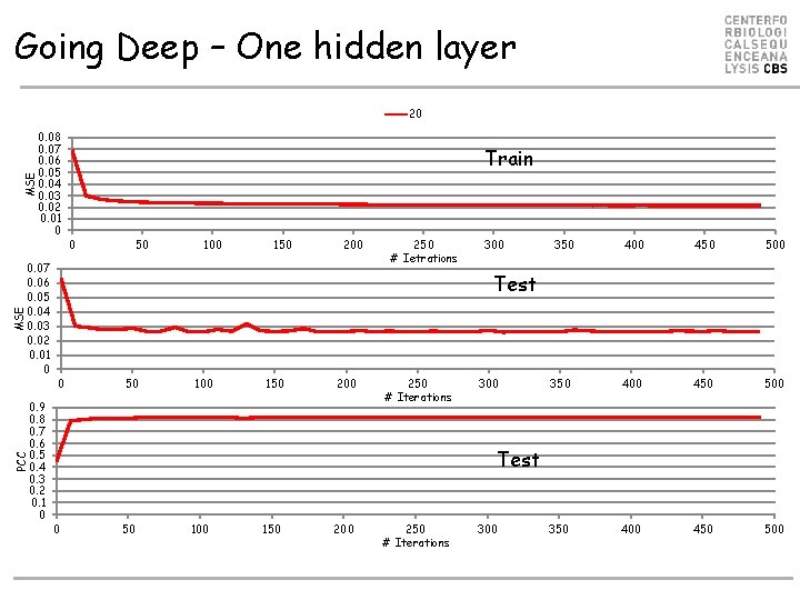
Going Deep – One hidden layer 20 Train MSE 0. 08 0. 07 0. 06 0. 05 0. 04 0. 03 0. 02 0. 01 0 50 100 150 200 250 # Ietrations 300 350 400 450 500 Test MSE 0. 07 0. 06 0. 05 0. 04 0. 03 0. 02 0. 01 0 0 50 100 150 200 250 # Iterations 300 Test PCC 0. 9 0. 8 0. 7 0. 6 0. 5 0. 4 0. 3 0. 2 0. 1 0 0 0 50 100 150 200 250 # Iterations 300

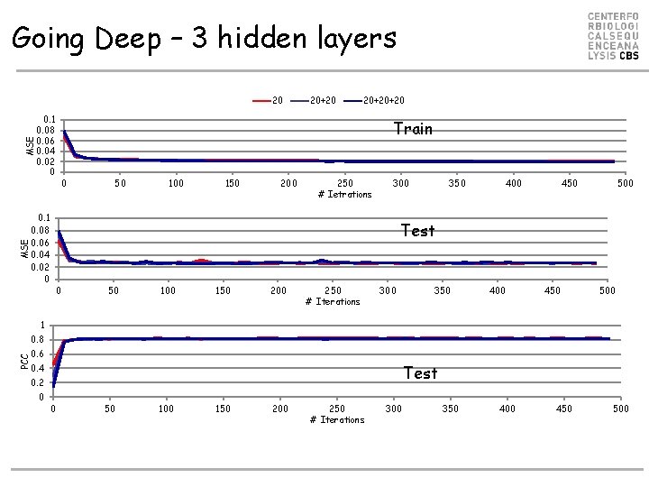
Going Deep – 3 hidden layers 20 20+20+20 Train MSE 0. 1 0. 08 0. 06 0. 04 0. 02 0 20+20 0. 1 0. 08 0. 06 0. 04 0. 02 0 0 50 100 150 200 250 # Ietrations 300 350 400 450 500 MSE Test 0 50 100 150 200 250 # Iterations 300 350 400 450 500 1 0. 8 PCC 0. 6 Test 0. 4 0. 2 0 0 50 100 150 200 250 # Iterations 300 350 400 450 500

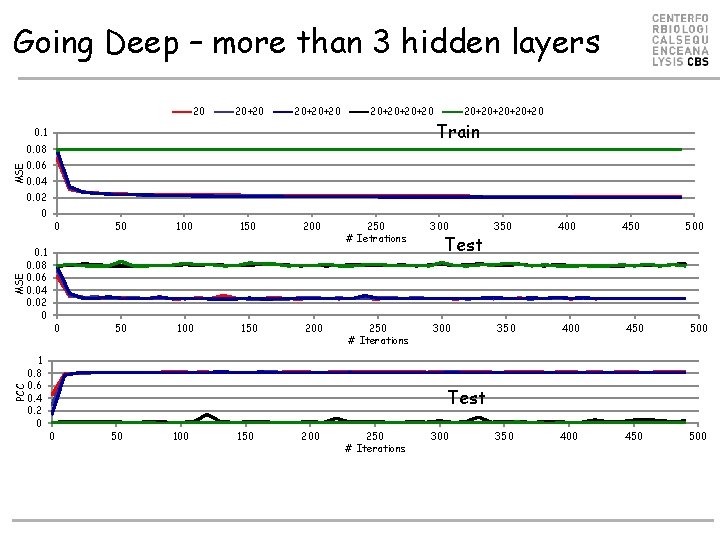
Going Deep – more than 3 hidden layers 20 20+20+20+20 0. 1 0. 08 20+20+20 Train MSE 0. 06 0. 04 0. 02 0 50 100 150 200 250 # Ietrations 300 0 50 100 150 200 250 # Iterations 300 Test 350 400 450 500 MSE 0. 1 0. 08 0. 06 0. 04 0. 02 0 0 PCC 1 0. 8 0. 6 0. 4 0. 2 0 350 400 450 500 Test 0 50 100 150 200 250 # Iterations 300

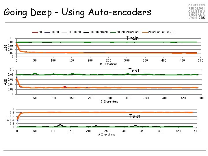
Going Deep – Using Auto-encoders 20 20+20+20+20+Auto Train MSE 0. 1 0. 08 0. 06 0. 04 0. 02 0 20+20 0 50 100 150 200 250 # Ietrations 300 350 400 450 500 Test 0. 1 0. 08 MSE 0. 06 0. 04 0. 02 0 50 100 150 200 250 # Iterations 300 350 400 450 500 Test PCC 1 0. 8 0. 6 0. 4 0. 2 0 0 0 50 100 150 200 250 # Iterations 300 350 400 450 500

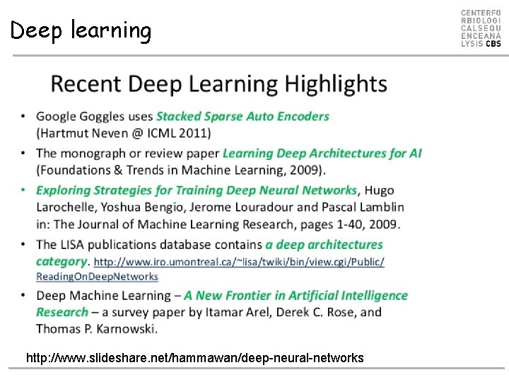
Deep learning http: //www. slideshare. net/hammawan/deep-neural-networks

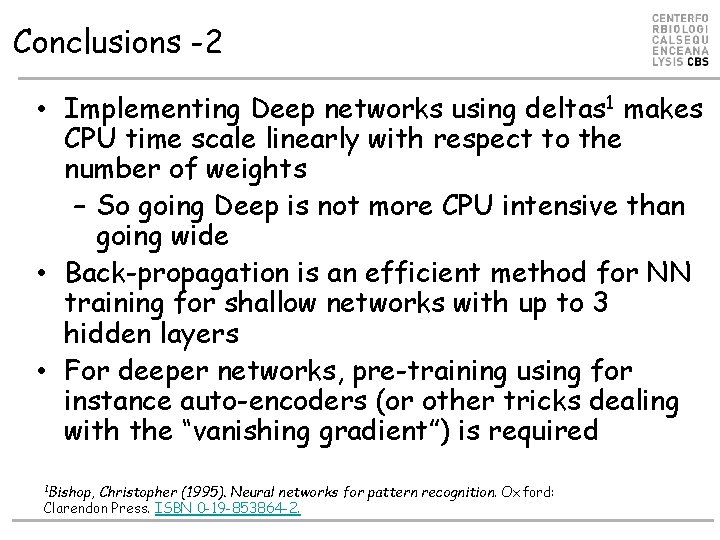
Conclusions -2 • Implementing Deep networks using deltas 1 makes CPU time scale linearly with respect to the number of weights – So going Deep is not more CPU intensive than going wide • Back-propagation is an efficient method for NN training for shallow networks with up to 3 hidden layers • For deeper networks, pre-training using for instance auto-encoders (or other tricks dealing with the “vanishing gradient”) is required 1 Bishop, Christopher (1995). Neural networks for pattern recognition. Oxford: Clarendon Press. ISBN 0 -19 -853864 -2.