ALGORITHMS NETWORK FLOW Uri Zwick Tel Aviv University

ALGORITHMS NETWORK FLOW Uri Zwick Tel Aviv University Reading material: Chapter 8 of Tarjan’s “Data structures and network algorithms” Chapter 26 of CLRS “Introduction to Algorithms”, third edition Last modified 07/07/2020

NETWORK FLOW Segment FLOW-1 Problem definition Problems modeled by network flow Network flow is an LP problem Cuts and flows

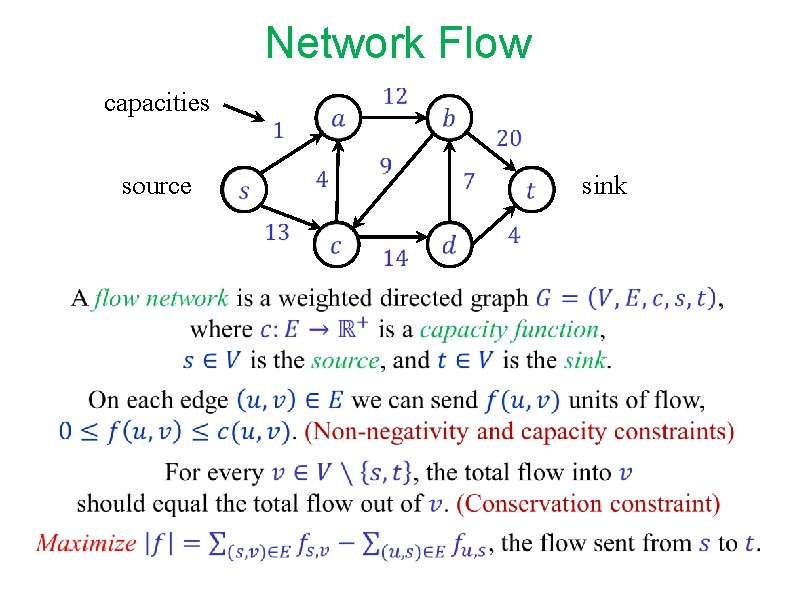
Network Flow capacities source sink

Problems modeled by Network Flow A variety of problems can be modeled by “Network Flow”: Liquids (water, oil, etc. ) flowing in pipe network. Goods shipped using a railroad network. Currents flowing in an electrical network. Information flowing through a communication network. We usually consider the rate of flow, i. e. , the amount of flow per unit of time. We consider steady state behavior. We ignore timing issues.

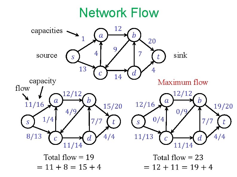
Network Flow capacities capacity flow source Maximum flow sink

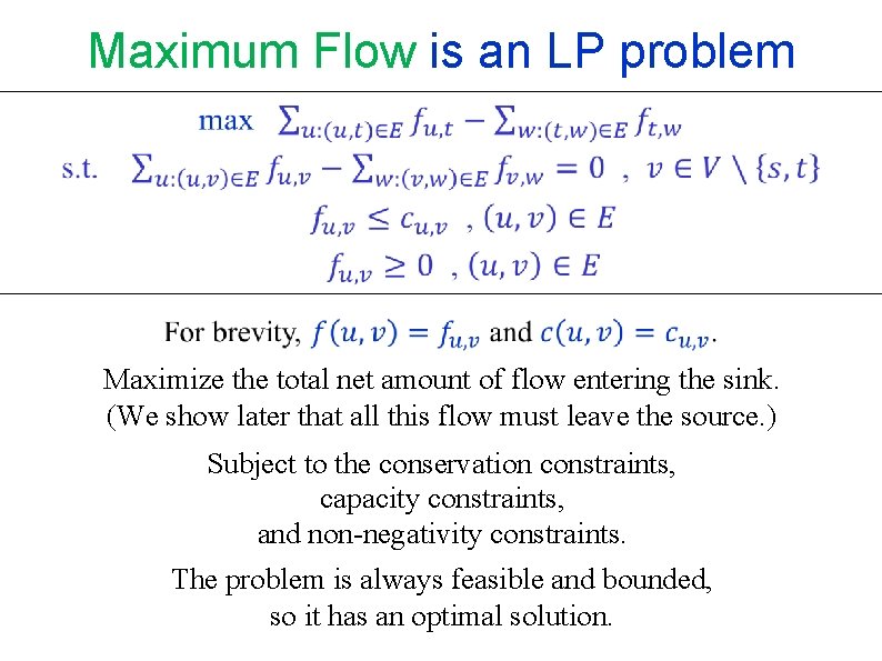
Maximum Flow is an LP problem Maximize the total net amount of flow entering the sink. (We show later that all this flow must leave the source. ) Subject to the conservation constraints, capacity constraints, and non-negativity constraints. The problem is always feasible and bounded, so it has an optimal solution.

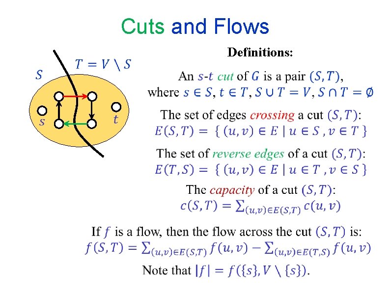
Cuts and Flows Definitions:

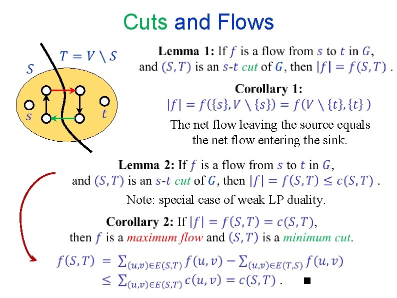
Cuts and Flows The net flow leaving the source equals the net flow entering the sink. Note: special case of weak LP duality.

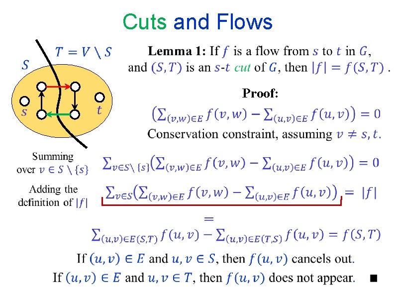
Cuts and Flows Proof:

END OF Segment FLOW-1

NETWORK FLOW Segment FLOW-2 Augmenting paths Augmenting flow along augmenting paths

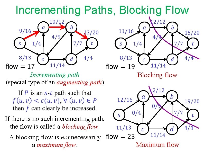
Incrementing Paths, Blocking Flow Incrementing path (special type of an augmenting path) A blocking flow is not necessarily a maximum flow. Blocking flow If there is no such incrementing path, the flow is called a blocking flow. Maximum flow

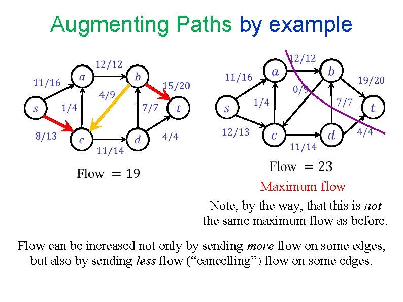
Augmenting Paths by example Maximum flow Note, by the way, that this is not the same maximum flow as before. Flow can be increased not only by sending more flow on some edges, but also by sending less flow (“cancelling”) flow on some edges.

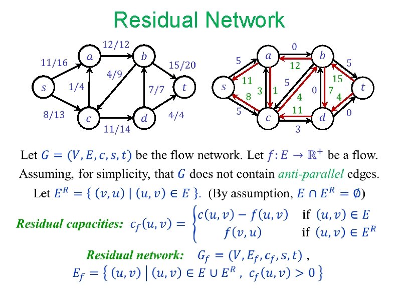
Residual Network

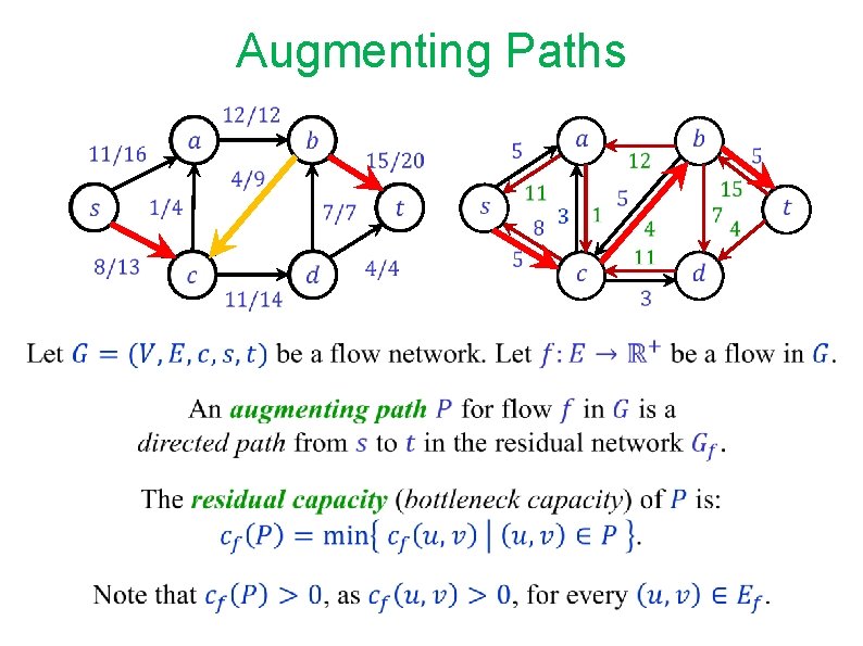
Augmenting Paths

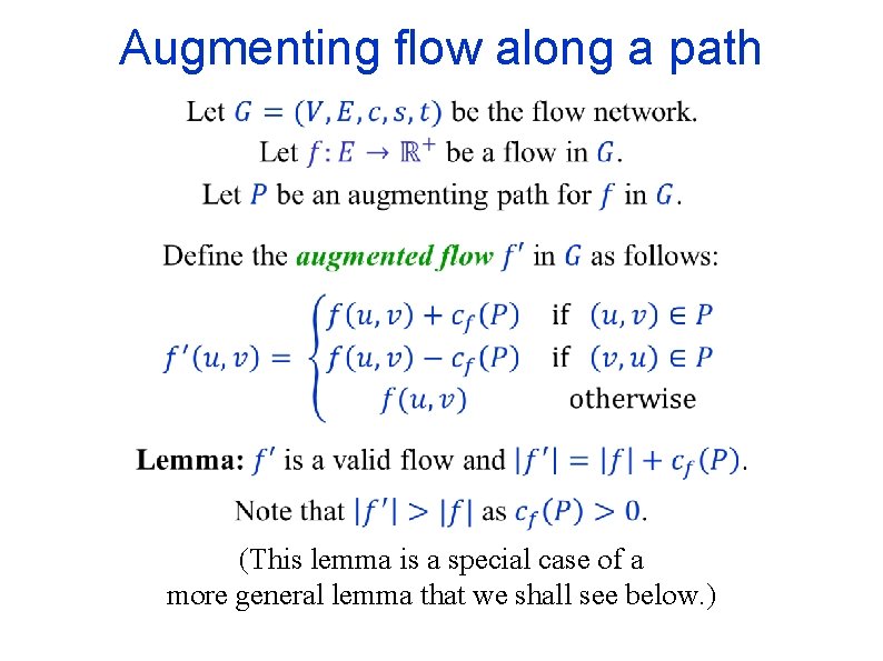
Augmenting flow along a path (This lemma is a special case of a more general lemma that we shall see below. )

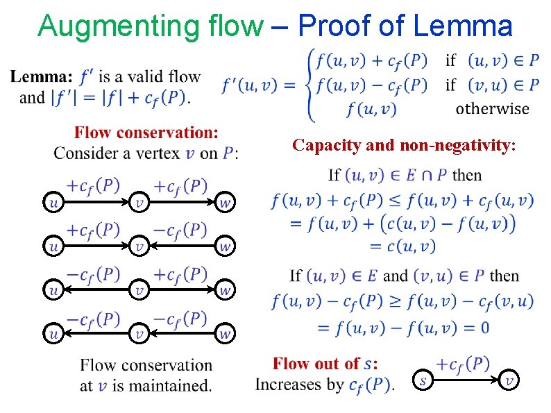
Augmenting flow – Proof of Lemma Capacity and non-negativity:

END OF Segment FLOW-2

NETWORK FLOW Segment FLOW-3 Maximum Flow Minimum Cut

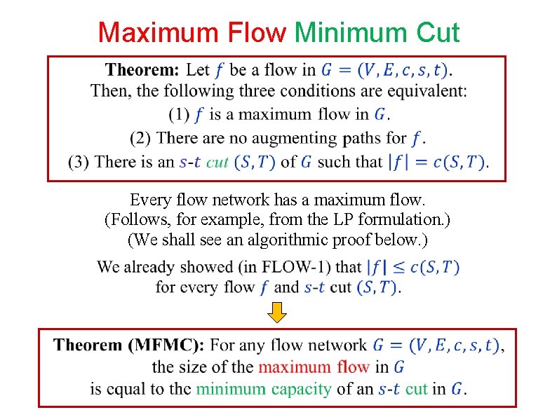
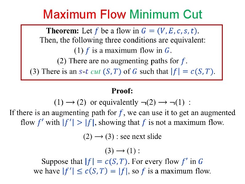
Maximum Flow Minimum Cut Every flow network has a maximum flow. (Follows, for example, from the LP formulation. ) (We shall see an algorithmic proof below. )

Maximum Flow Minimum Cut Proof:

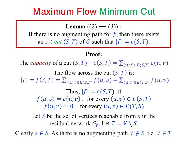
Maximum Flow Minimum Cut Proof:

Maximum Flow Minimum Cut Proof: (continued)

END OF Segment FLOW-3

NETWORK FLOW Segment FLOW-4 The Ford-Fulkerson method

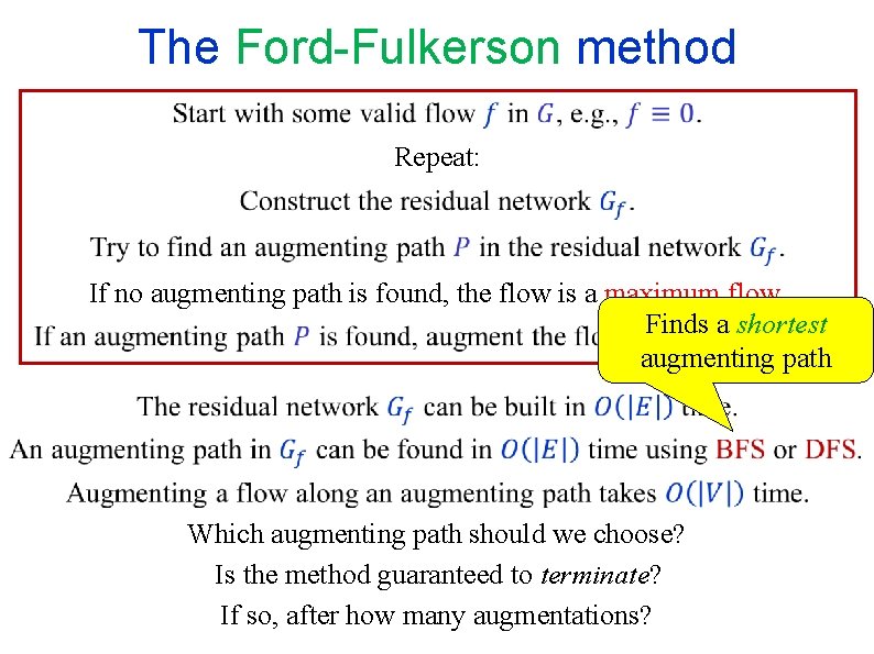
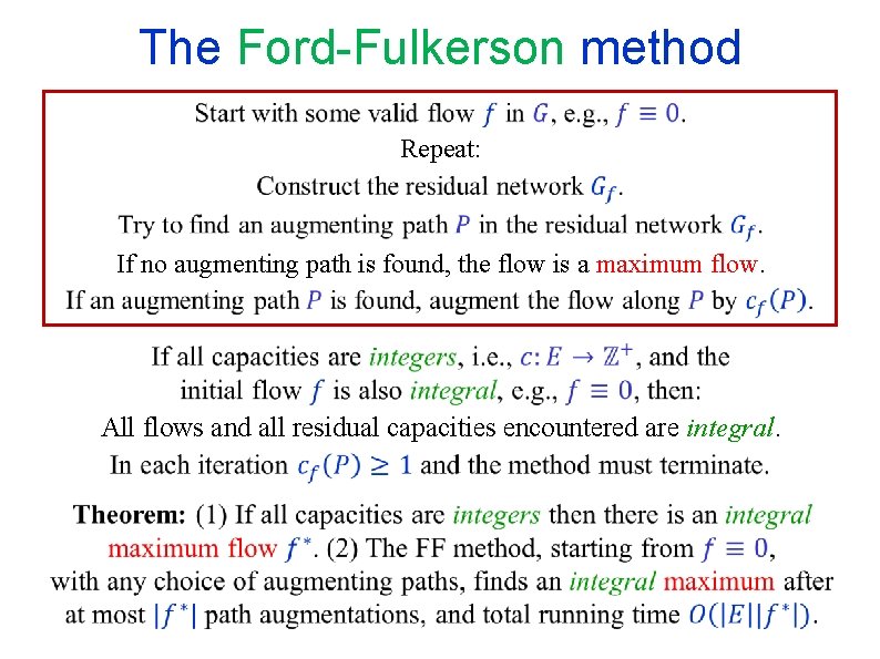
The Ford-Fulkerson method Repeat: If no augmenting path is found, the flow is a maximum flow. Finds a shortest augmenting path Which augmenting path should we choose? Is the method guaranteed to terminate? If so, after how many augmentations?

The Ford-Fulkerson method Repeat: If no augmenting path is found, the flow is a maximum flow. All flows and all residual capacities encountered are integral.

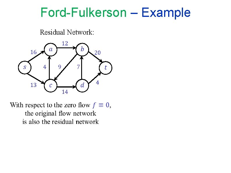
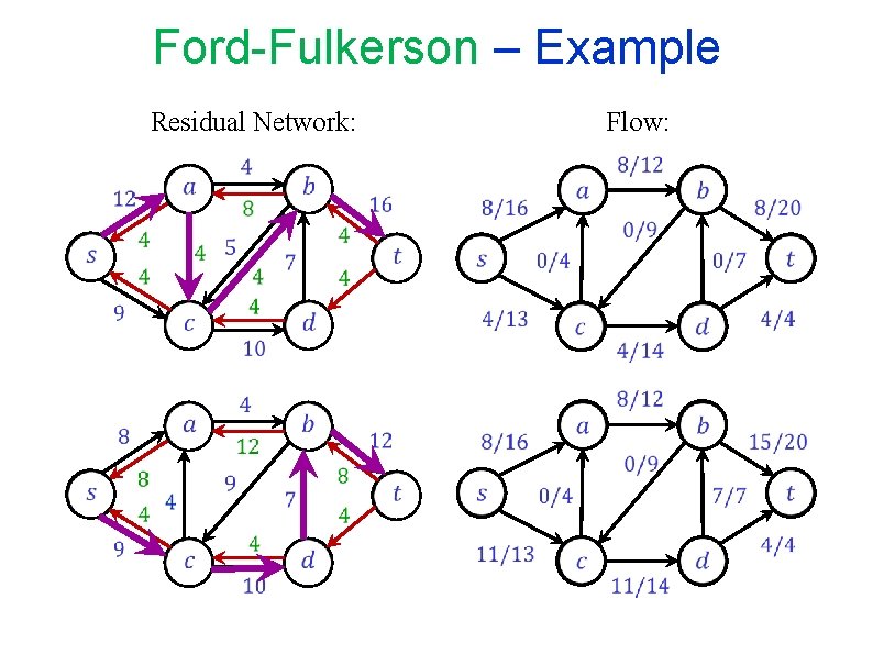
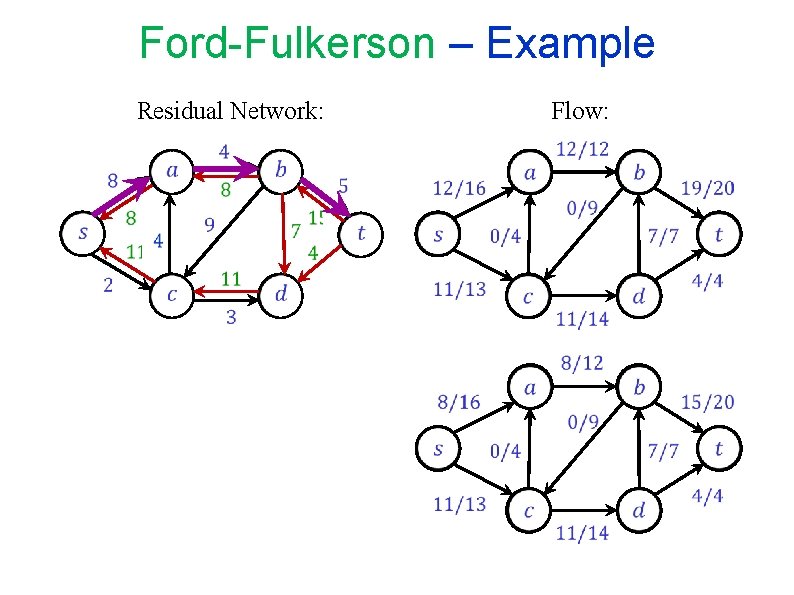
Ford-Fulkerson – Example Residual Network:

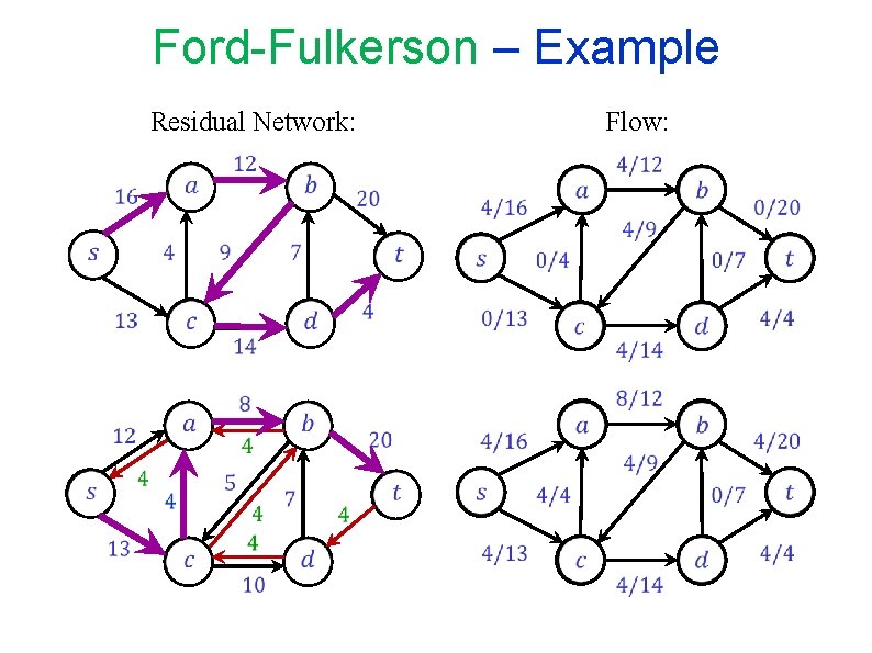
Ford-Fulkerson – Example Flow: Residual Network:

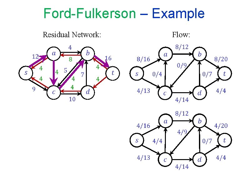
Ford-Fulkerson – Example Flow: Residual Network:

Ford-Fulkerson – Example Flow: Residual Network:

Ford-Fulkerson – Example Flow: Residual Network:

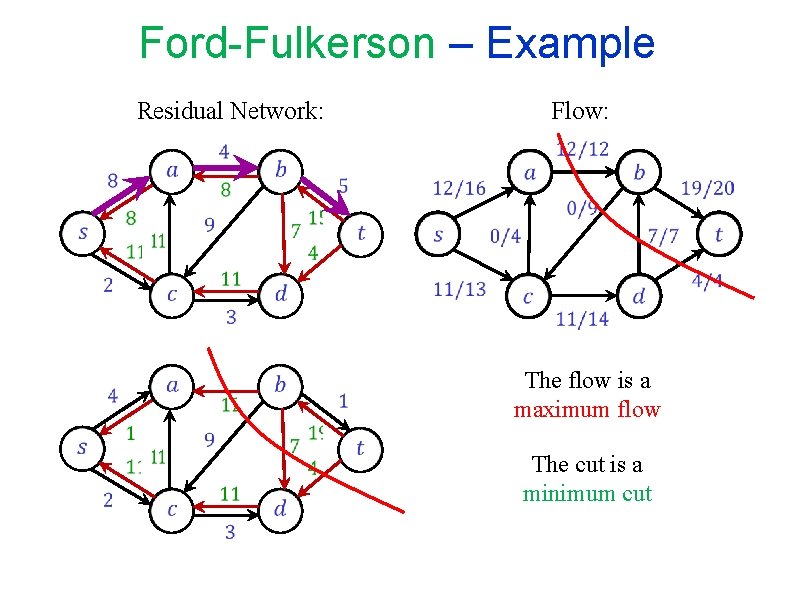
Ford-Fulkerson – Example Flow: Residual Network: The flow is a maximum flow The cut is a minimum cut

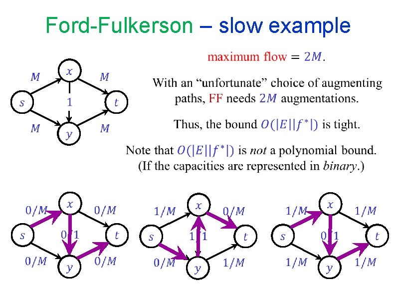
Ford-Fulkerson – slow example

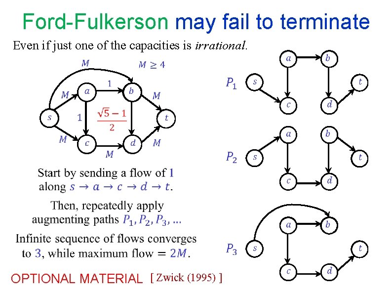
Ford-Fulkerson may fail to terminate Even if just one of the capacities is irrational. OPTIONAL MATERIAL [ Zwick (1995) ]

END OF Segment FLOW-4

NETWORK FLOW Segment FLOW-5 Bipartite matching

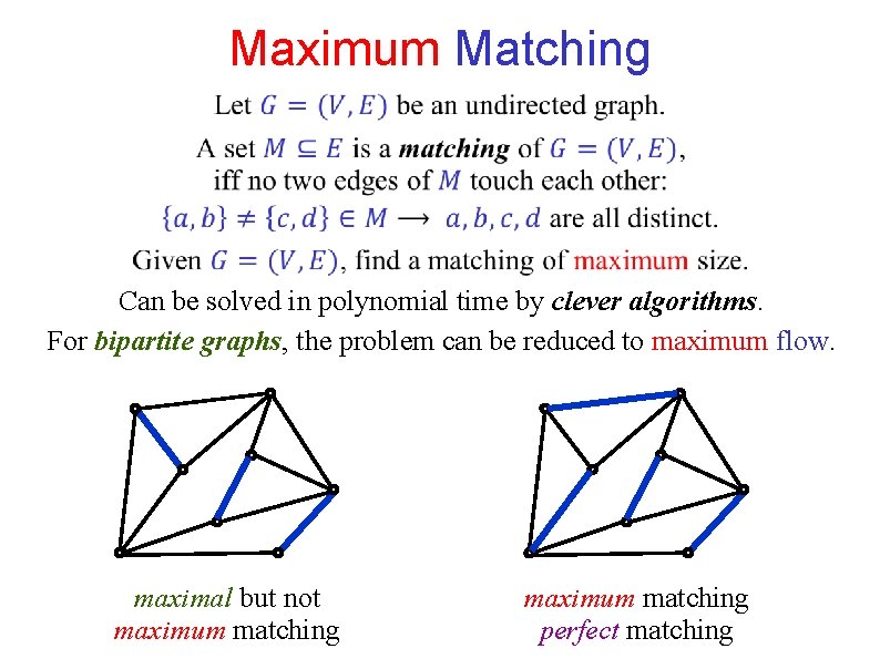
Maximum Matching Can be solved in polynomial time by clever algorithms. For bipartite graphs, the problem can be reduced to maximum flow. maximal but not maximum matching perfect matching

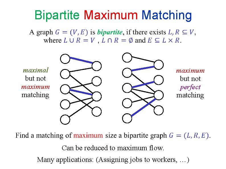
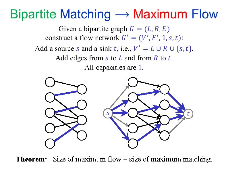
Bipartite Maximum Matching maximal but not maximum matching maximum but not perfect matching Can be reduced to maximum flow. Many applications: (Assigning jobs to workers, …)

All capacities are 1. Theorem: Size of maximum flow = size of maximum matching.

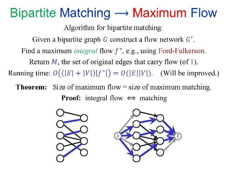
Algorithm for bipartite matching: Theorem: Size of maximum flow = size of maximum matching.

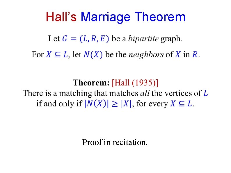
Hall’s Marriage Theorem Proof in recitation.

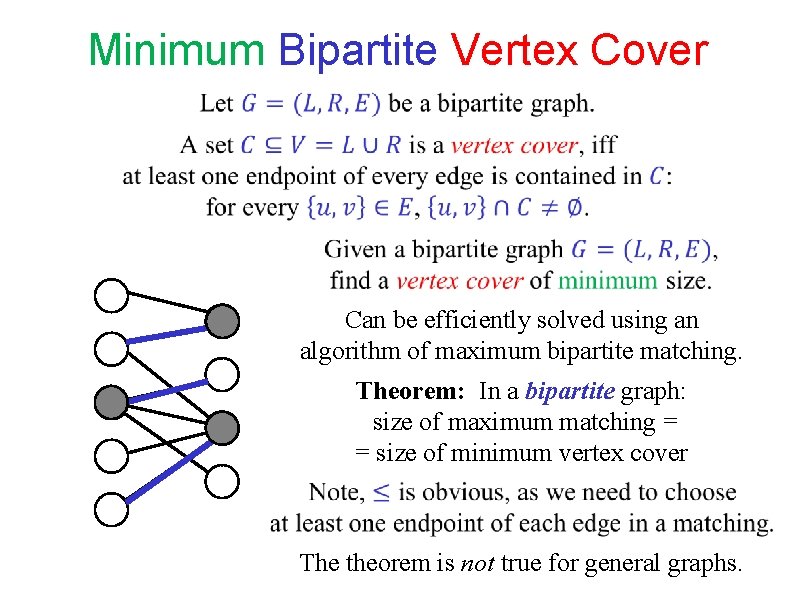
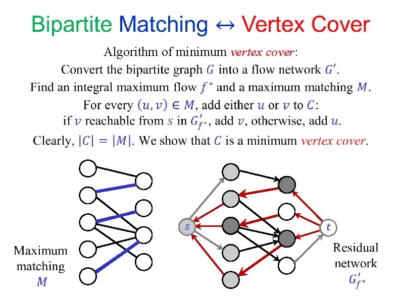
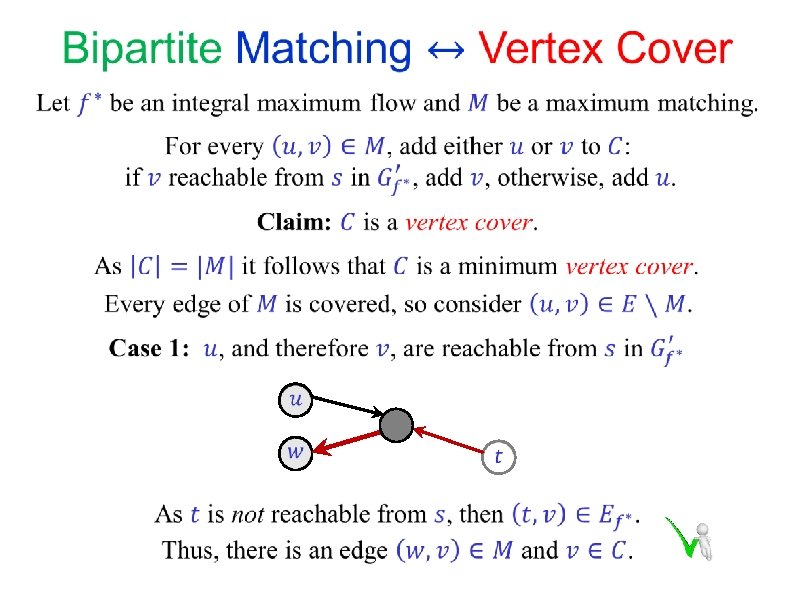
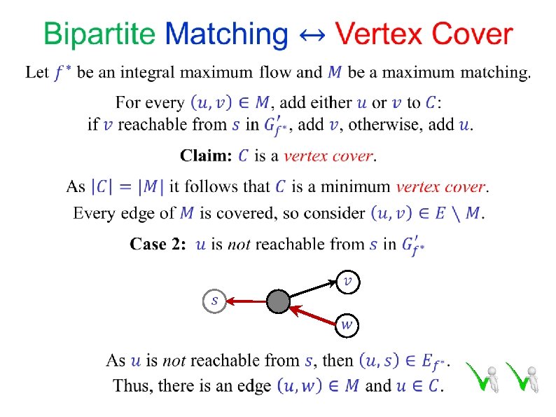
Minimum Bipartite Vertex Cover Can be efficiently solved using an algorithm of maximum bipartite matching. Theorem: In a bipartite graph: size of maximum matching = = size of minimum vertex cover The theorem is not true for general graphs.

Algorithm of minimum vertex cover:

END OF Segment FLOW-5

NETWORK FLOW Segment FLOW-6 The Edmond-Karp algorithm(s) (1972) By Jeff. AEdmonds - Own work, CC BY-SA 4. 0, https: //commons. wikimedia. org/w/index. php? c urid=87019881

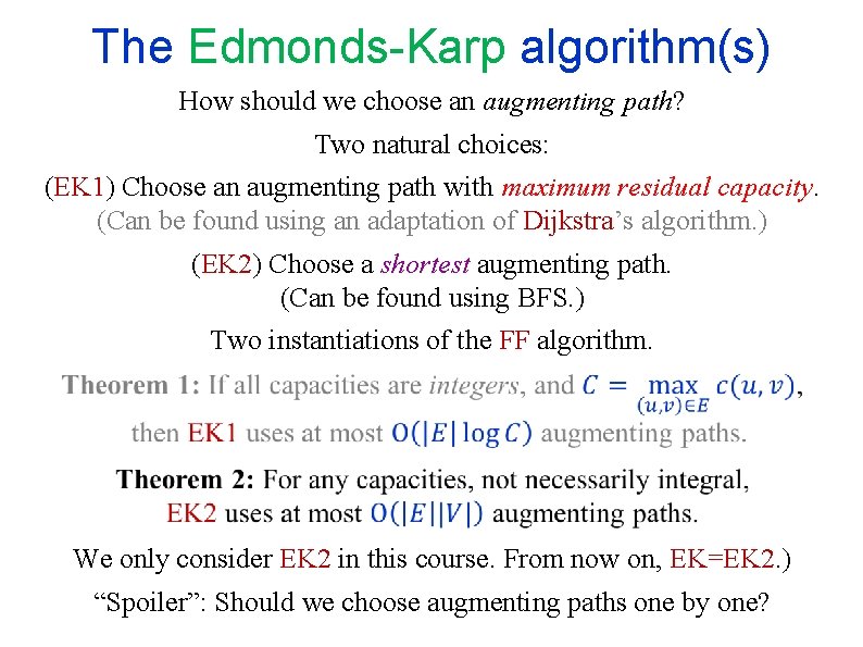
The Edmonds-Karp algorithm(s) How should we choose an augmenting path? Two natural choices: (EK 1) Choose an augmenting path with maximum residual capacity. (Can be found using an adaptation of Dijkstra’s algorithm. ) (EK 2) Choose a shortest augmenting path. (Can be found using BFS. ) Two instantiations of the FF algorithm. We only consider EK 2 in this course. From now on, EK=EK 2. ) “Spoiler”: Should we choose augmenting paths one by one?

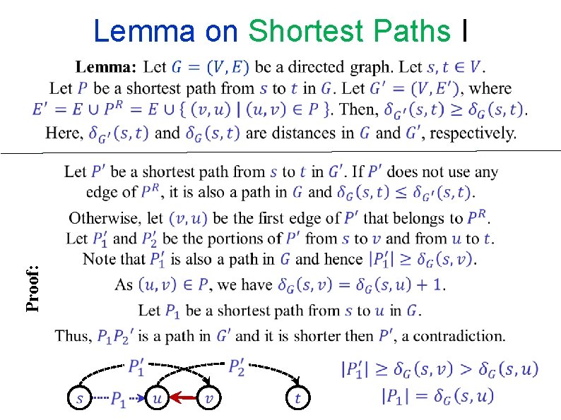
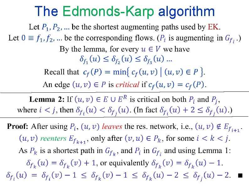
Lemma on Shortest Paths I Proof:

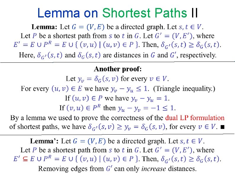
Lemma on Shortest Paths II Another proof:

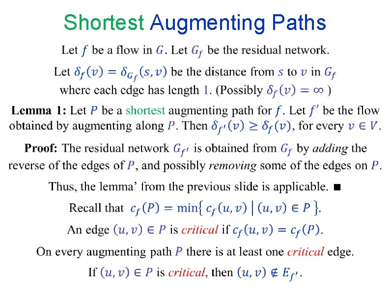
Shortest Augmenting Paths

The Edmonds-Karp algorithm

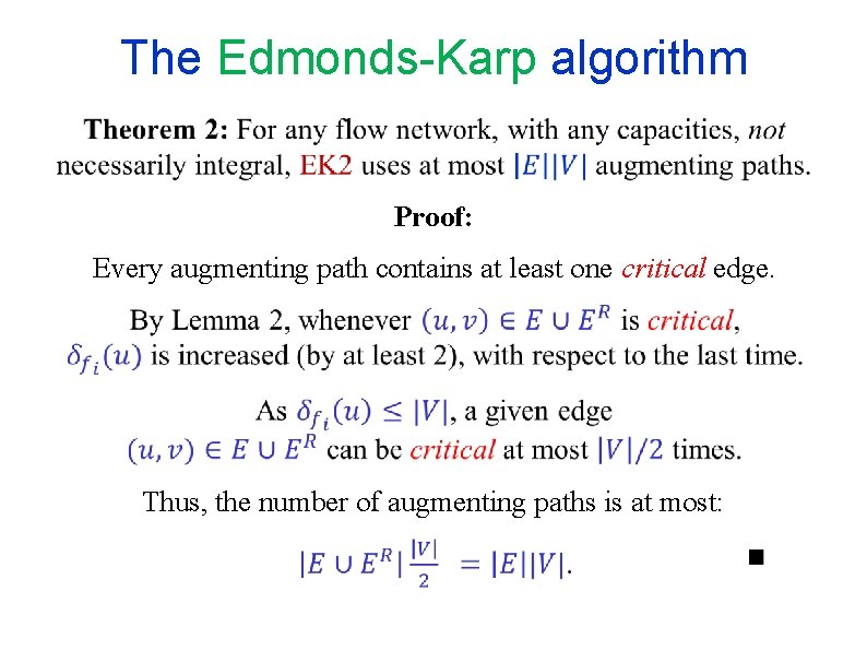
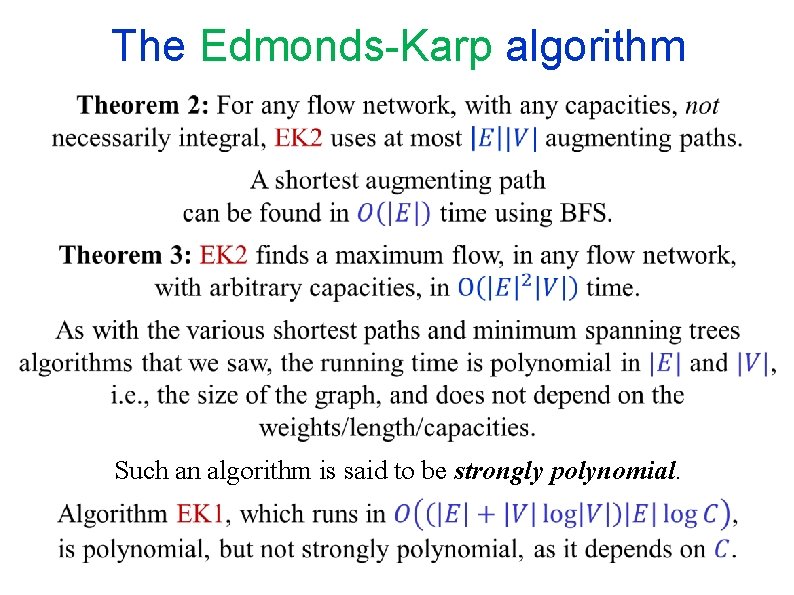
The Edmonds-Karp algorithm Proof: Every augmenting path contains at least one critical edge. Thus, the number of augmenting paths is at most:

The Edmonds-Karp algorithm Such an algorithm is said to be strongly polynomial.

END OF Segment FLOW-6

NETWORK FLOW Segment FLOW-7 Edmonds-Karp - Examples

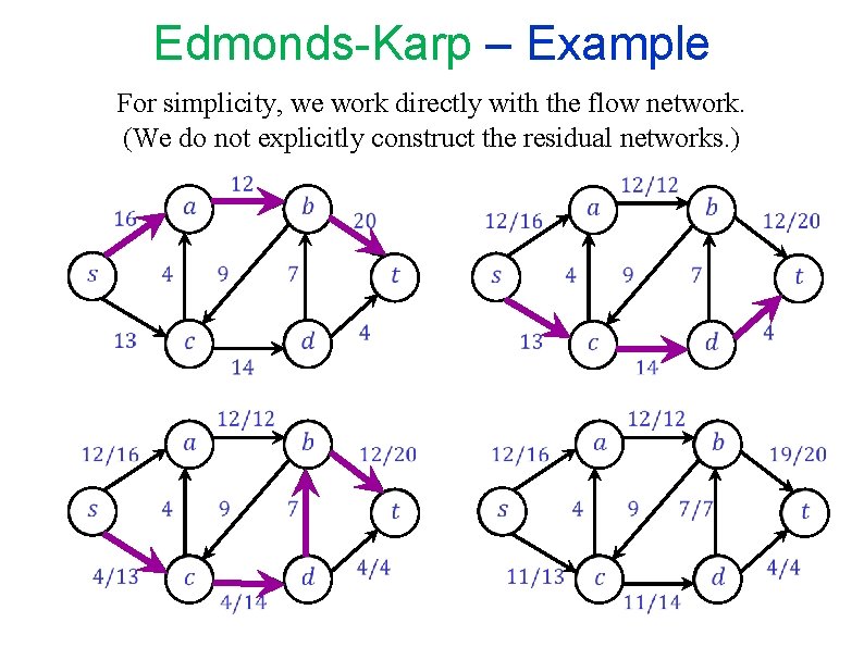
Edmonds-Karp – Example For simplicity, we work directly with the flow network. (We do not explicitly construct the residual networks. )

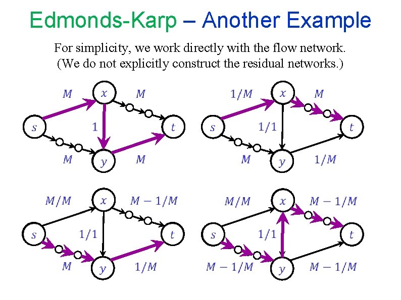
Edmonds-Karp – Another Example For simplicity, we work directly with the flow network. (We do not explicitly construct the residual networks. )

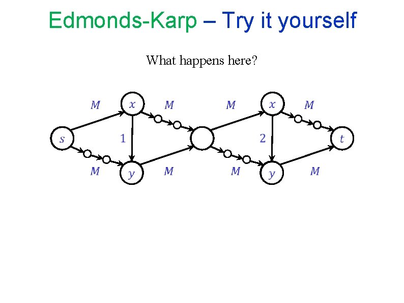
Edmonds-Karp – Try it yourself What happens here?

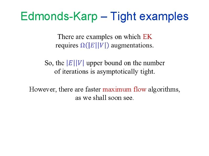
Edmonds-Karp – Tight examples However, there are faster maximum flow algorithms, as we shall soon see.

END OF Segment FLOW-7

NETWORK FLOW Segment FLOW-8 Residual flows “Adding” and “Subtracting” flows More general flow augmentations

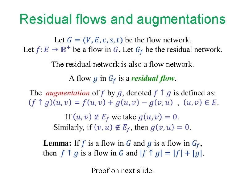
Residual flows and augmentations The residual network is also a flow network. Proof on next slide.

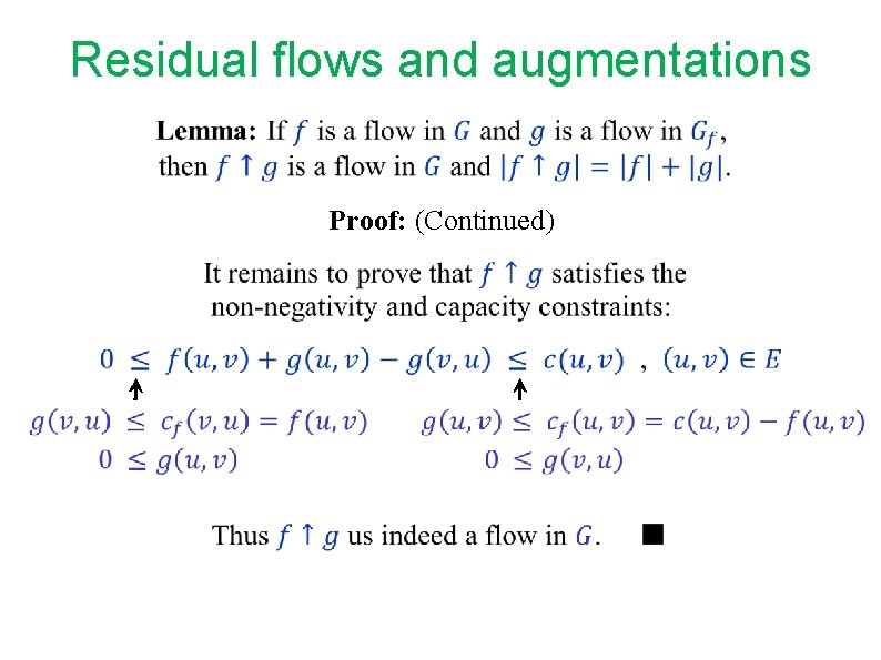
Residual flows and augmentations

Residual flows and augmentations Proof: (Continued)

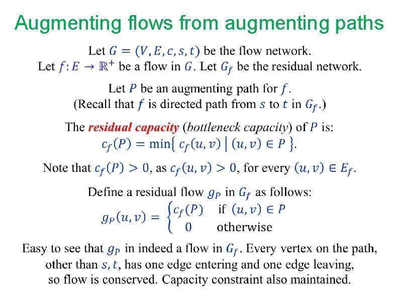
Augmenting flows from augmenting paths

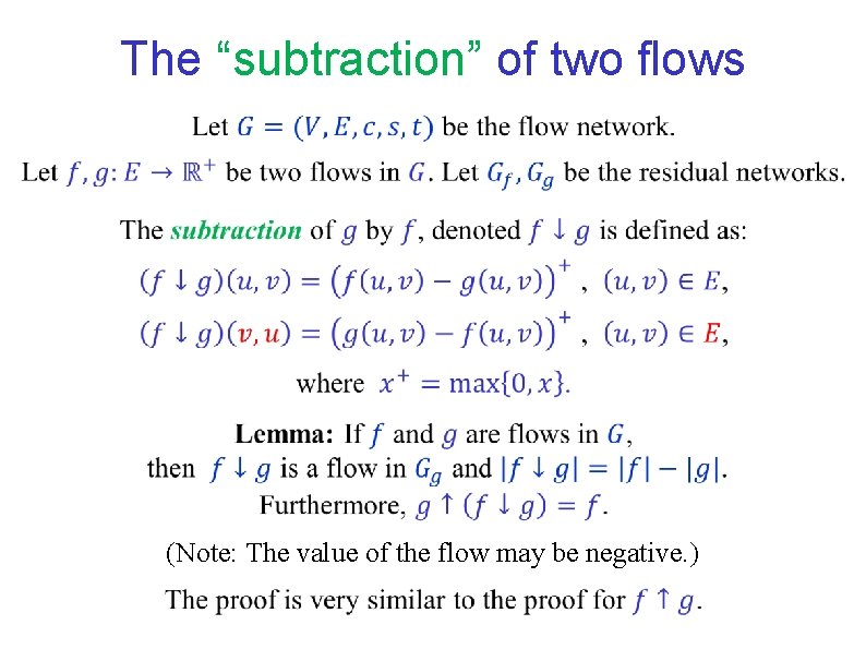
The “subtraction” of two flows (Note: The value of the flow may be negative. )

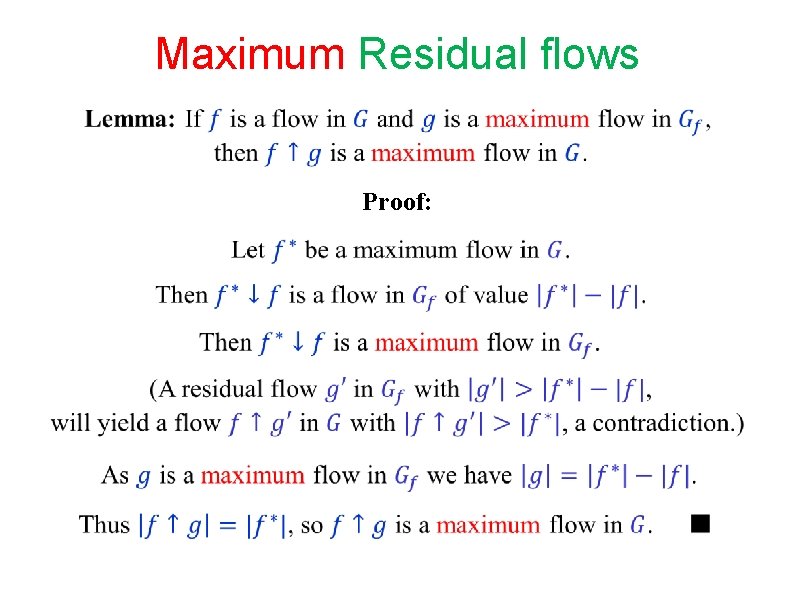
Maximum Residual flows Proof:

END OF Segment FLOW-8

NETWORK FLOW Segment FLOW-9 Dinic’s algorithm (1970) Yefim Dinitz

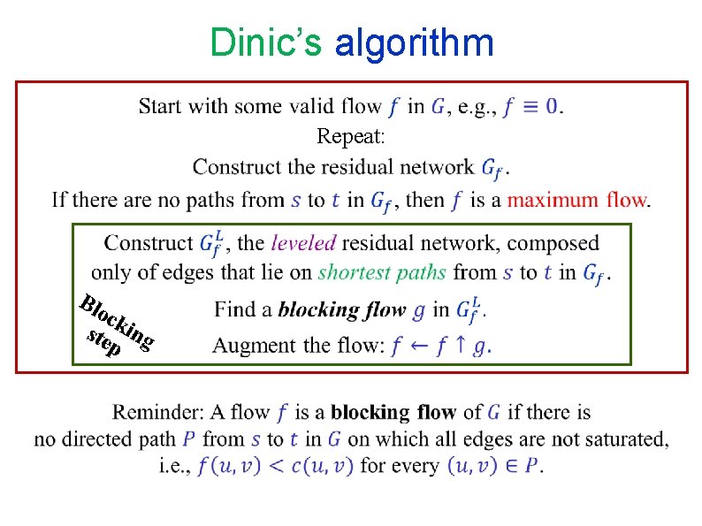
Dinic’s algorithm Repeat: Blo ck ste ing p

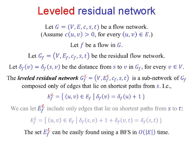
Leveled residual network

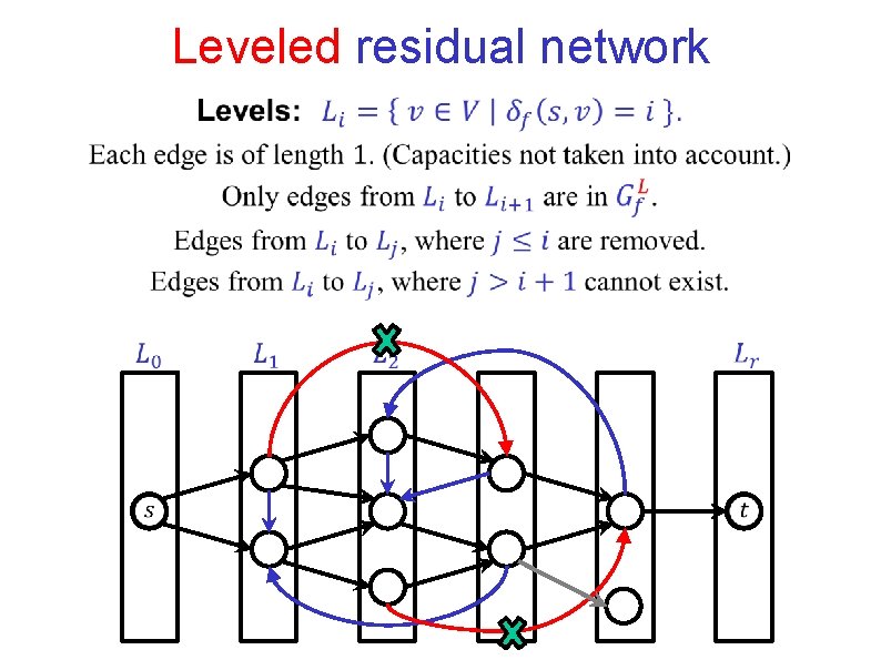
Leveled residual network

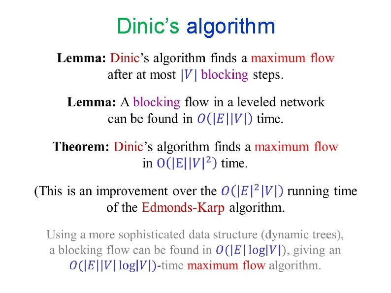
Dinic’s algorithm

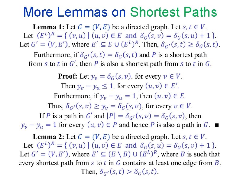
More Lemmas on Shortest Paths

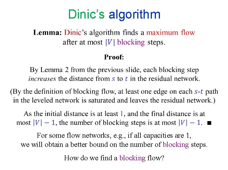
Dinic’s algorithm Proof: For some flow networks, e. g. , if all capacities are 1, we will obtain a better bound on the number of blocking steps. How do we find a blocking flow?

END OF Segment FLOW-9

NETWORK FLOW Segment FLOW-10 Finding blocking flows

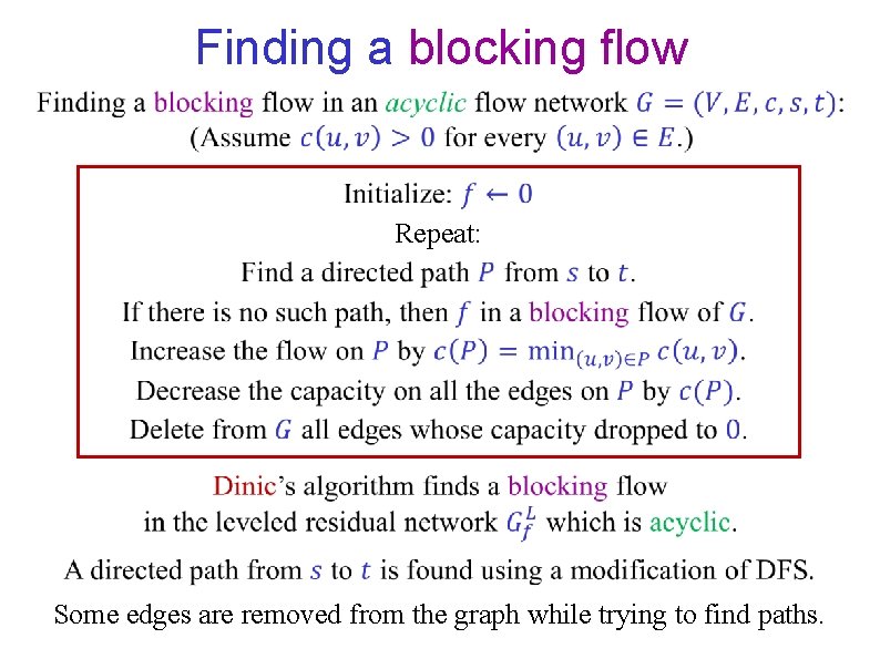
Finding a blocking flow Repeat: Some edges are removed from the graph while trying to find paths.

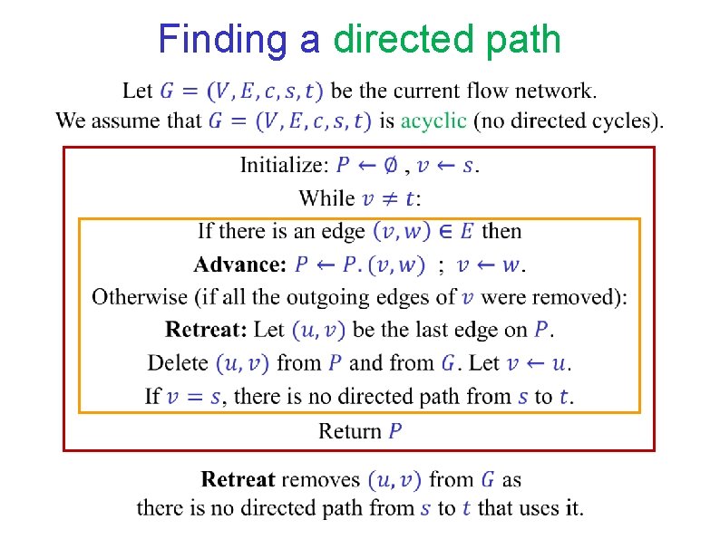
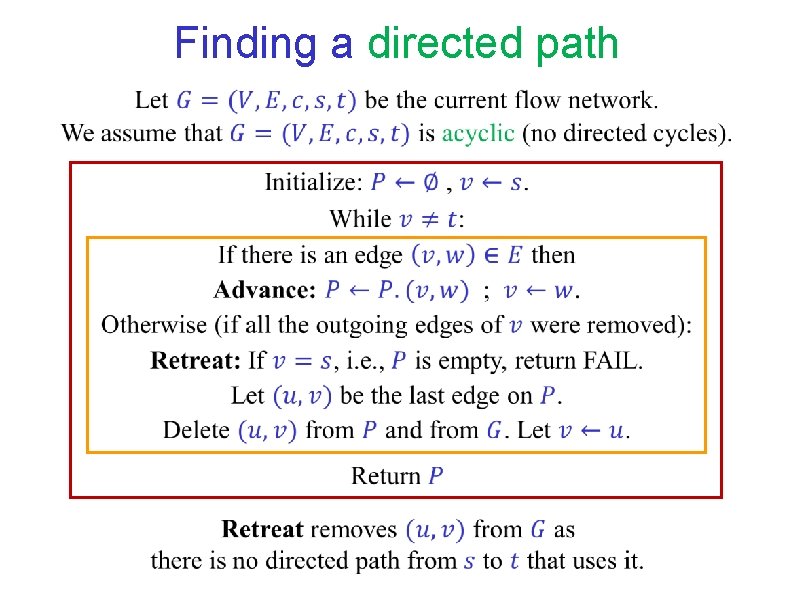
Finding a directed path

Finding a directed path

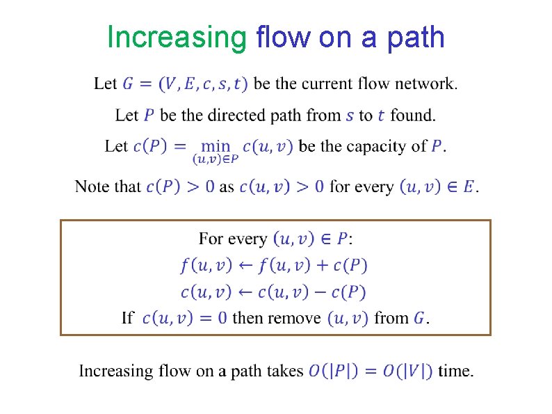
Increasing flow on a path

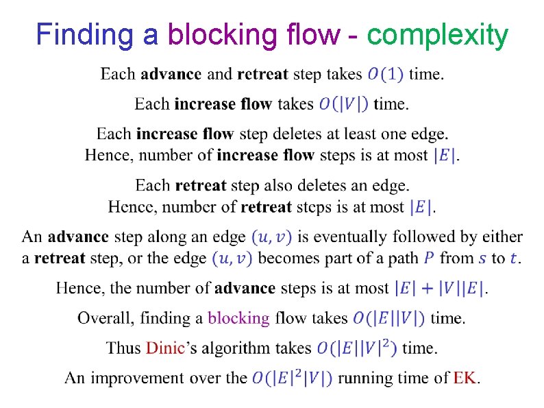
Finding a blocking flow - complexity

END OF Segment FLOW-10

NETWORK FLOW Segment FLOW-11 Dinic’s algorithm in unit networks

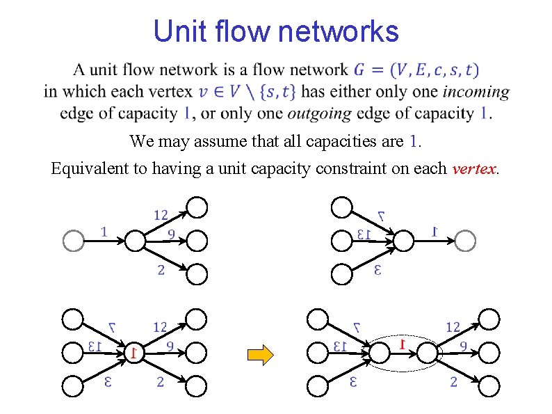
Unit flow networks We may assume that all capacities are 1. Equivalent to having a unit capacity constraint on each vertex.

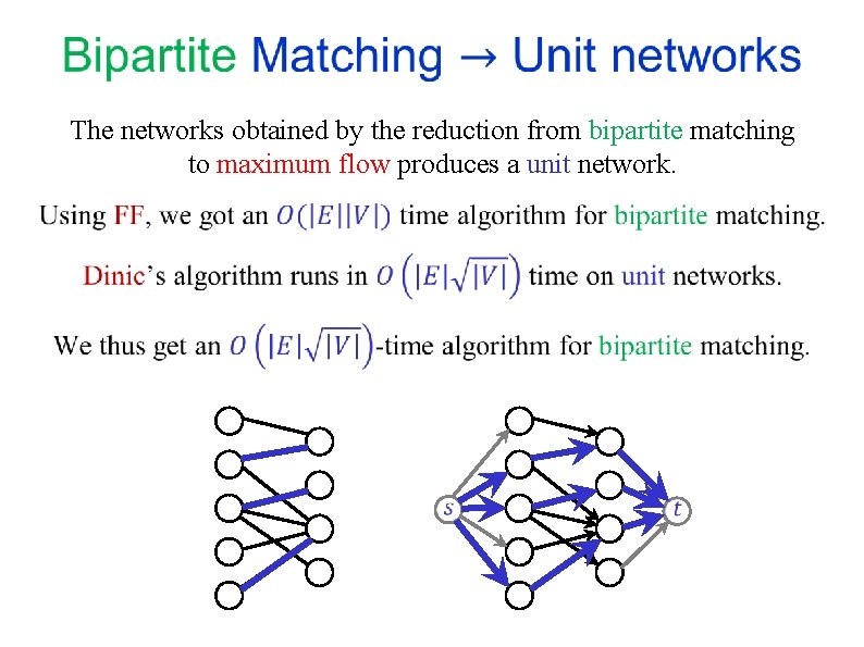
The networks obtained by the reduction from bipartite matching to maximum flow produces a unit network.

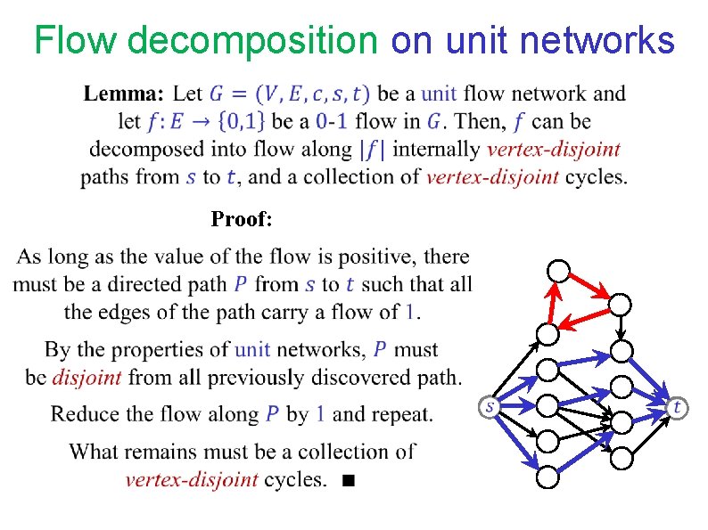
Flow decomposition on unit networks Proof:

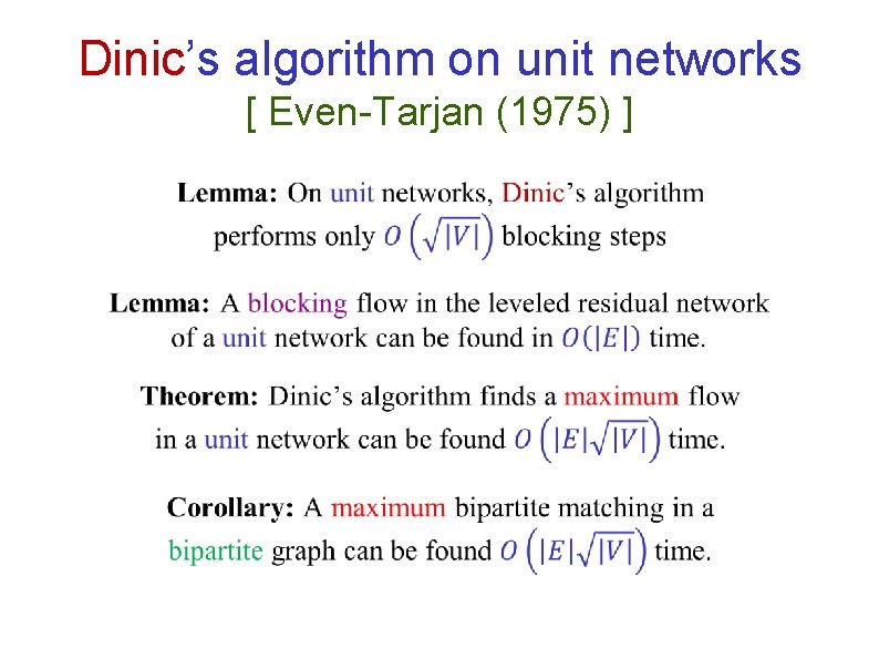
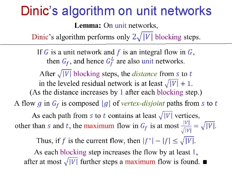
Dinic’s algorithm on unit networks [ Even-Tarjan (1975) ]

Dinic’s algorithm on unit networks

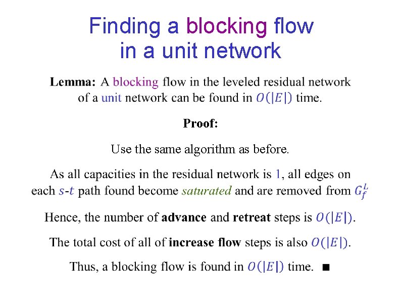
Finding a blocking flow in a unit network Proof: Use the same algorithm as before.

END OF Segment FLOW-11

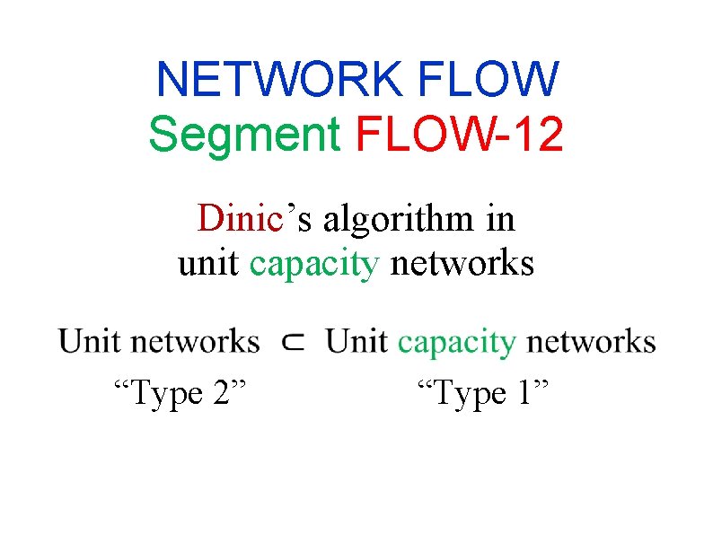
NETWORK FLOW Segment FLOW-12 Dinic’s algorithm in unit capacity networks “Type 2” “Type 1”

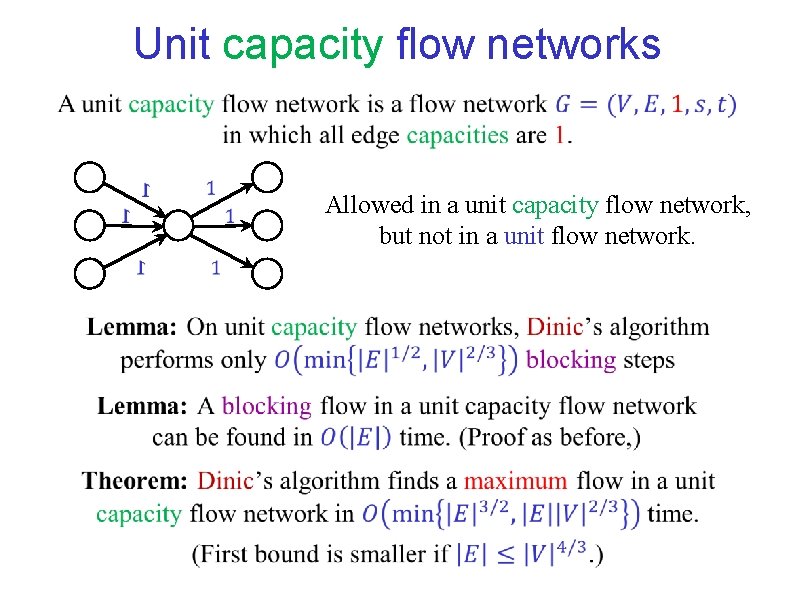
Unit capacity flow networks Allowed in a unit capacity flow network, but not in a unit flow network.

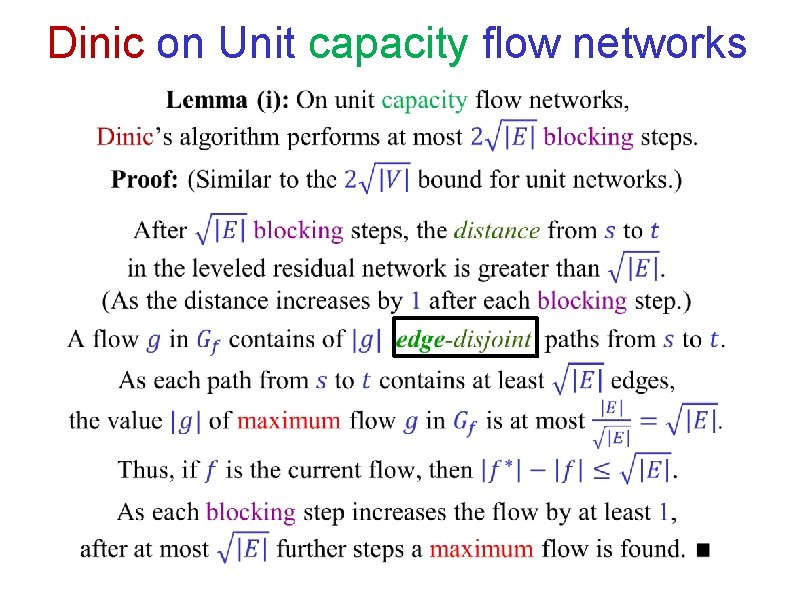
Dinic on Unit capacity flow networks

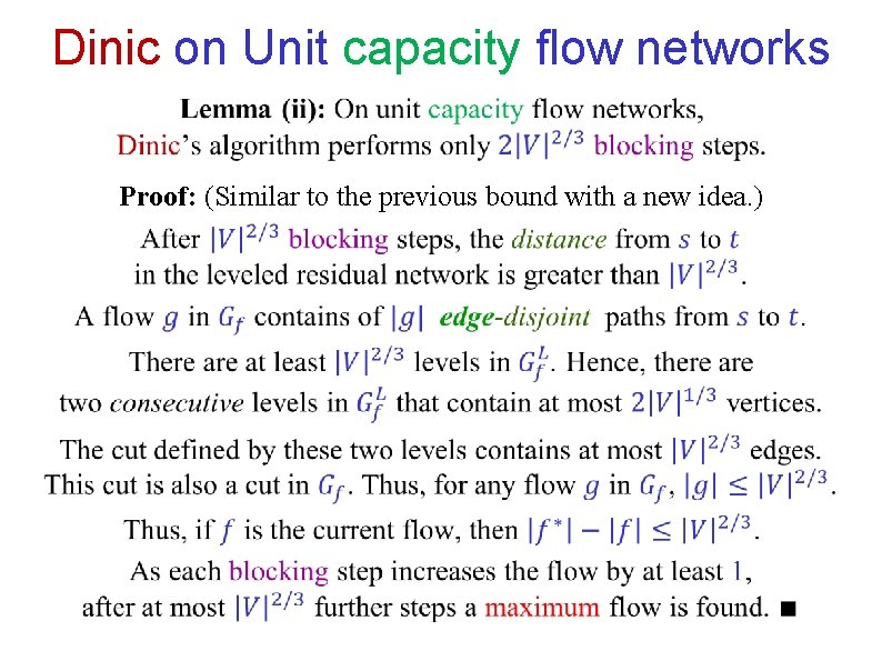
Dinic on Unit capacity flow networks Proof: (Similar to the previous bound with a new idea. )

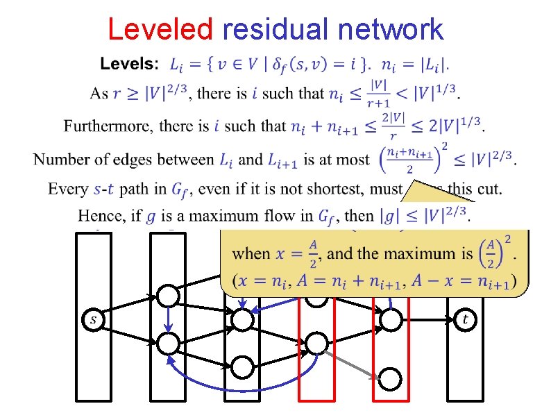
Leveled residual network

END OF Segment FLOW-12

NETWORK FLOW Segment FLOW-13 Allowing anti-parallel edges

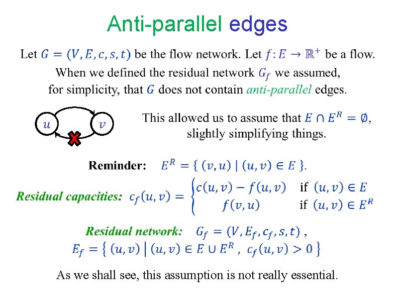
Anti-parallel edges As we shall see, this assumption is not really essential.

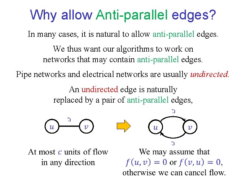
Why allow Anti-parallel edges? In many cases, it is natural to allow anti-parallel edges. We thus want our algorithms to work on networks that may contain anti-parallel edges. Pipe networks and electrical networks are usually undirected. An undirected edge is naturally replaced by a pair of anti-parallel edges,

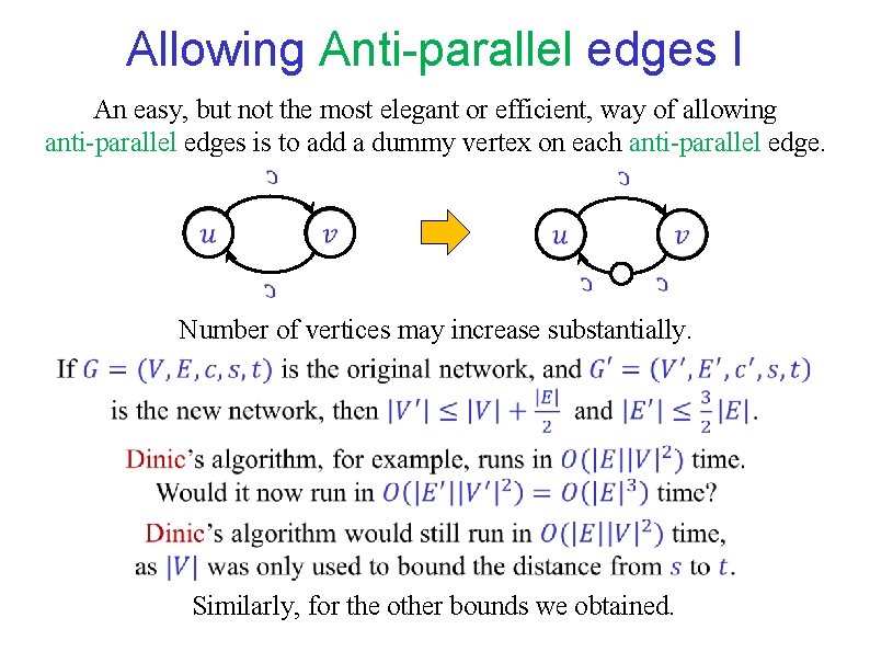
Allowing Anti-parallel edges I An easy, but not the most elegant or efficient, way of allowing anti-parallel edges is to add a dummy vertex on each anti-parallel edge. Number of vertices may increase substantially. Similarly, for the other bounds we obtained.

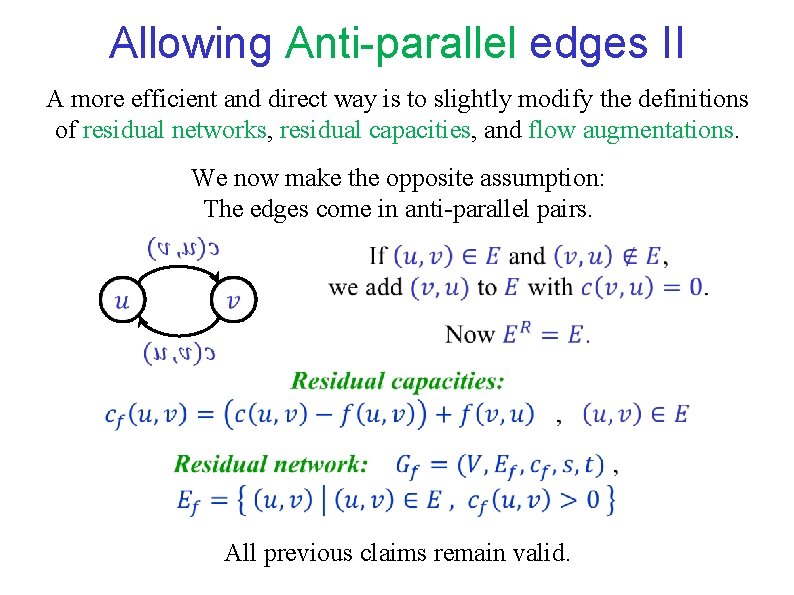
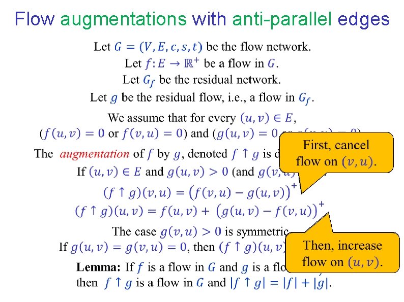
Allowing Anti-parallel edges II A more efficient and direct way is to slightly modify the definitions of residual networks, residual capacities, and flow augmentations. We now make the opposite assumption: The edges come in anti-parallel pairs. All previous claims remain valid.

Flow augmentations with anti-parallel edges

END OF Segment FLOW-13

NETWORK FLOW Segment FLOW-14 Flows as skew-symmetric functions

Flows as skew-symmetric functions

END OF Segment FLOW-14