Algorithm An algorithm is a set of instructions

Algorithm • An algorithm is a set of instructions to be followed to solve a problem. – There can be more than one solution (more than one algorithm) to solve a given problem. – An algorithm can be implemented using different programming languages on different platforms. • An algorithm must be correct. It should correctly solve the problem. • Once we have a correct algorithm for a problem, we have to determine the efficiency of that algorithm. – how much time that algorithm requires. – how much space that algorithm requires. • We will focus: – How to estimate the time required for an algorithm – How to reduce the time required 12/2/2020 CS 202 - Fundamentals of Computer Science II 1

Analysis of Algorithms • We can have different algorithms to solve a given problem. Which one is the most efficient? Between the given two algorithms, which one is more efficient? • Analysis of Algorithms is the area of computer science that provides tools to analyze the efficiency of different methods of solutions. • The efficiency of an algorithm means – – How much time it requires. How much memory space it requires. How much disk space and other resources it requires. We will concentrate on the time requirement. • We will try to find the efficiency of the algorithms, not their implementations. • An analysis should focus on gross differences in the efficiency of algorithms that are likely to dominate the overall cost of a solution. 12/2/2020 CS 202 - Fundamentals of Computer Science II 2

Analysis of Algorithms (cont. ) • How do we compare the time efficiency of two algorithms that solve the same problem? Naïve Approach: To implement these algorithms in a programming language (C++), and run them to compare their time requirements. Comparing the programs (instead of algorithms) has difficulties. • How are the algorithms coded? – Comparing running times means comparing the implementations. – We should not compare implementations, because they are sensitive to programming style that may cloud the issue of which algorithm is inherently more efficient. • What computer should we use? – We should compare the efficiency of the algorithms independently of a particular computer. • What data should the program use? – Any analysis must be independent of specific data. 12/2/2020 CS 202 - Fundamentals of Computer Science II 3

Analysis of Algorithms (cont. ) • When we analyze algorithms, we should employ mathematical techniques that analyze algorithms independently of specific implementations, computers, or data. • To analyze algorithms: – First, we start the count the number of significant operations in a particular solution to assess its efficiency. – Then, we will express the efficiency of algorithms using growth functions. 12/2/2020 CS 202 - Fundamentals of Computer Science II 4

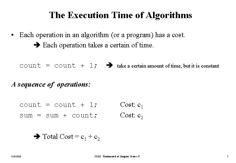
The Execution Time of Algorithms • Each operation in an algorithm (or a program) has a cost. Each operation takes a certain of time. count = count + 1; take a certain amount of time, but it is constant A sequence of operations: count = count + 1; sum = sum + count; Cost: c 1 Cost: c 2 Total Cost = c 1 + c 2 12/2/2020 CS 202 - Fundamentals of Computer Science II 5

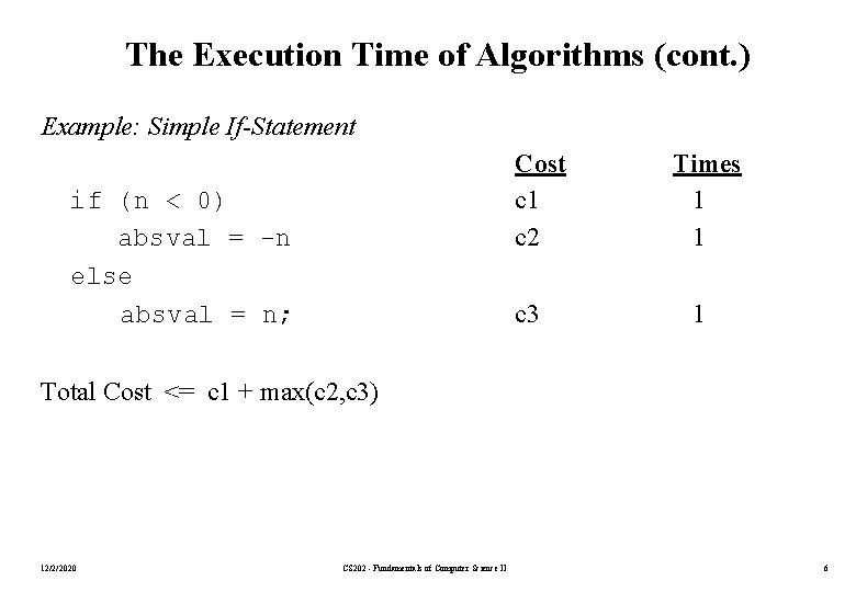
The Execution Time of Algorithms (cont. ) Example: Simple If-Statement if (n < 0) absval = -n else absval = n; Cost c 1 c 2 Times 1 1 c 3 1 Total Cost <= c 1 + max(c 2, c 3) 12/2/2020 CS 202 - Fundamentals of Computer Science II 6

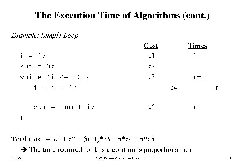
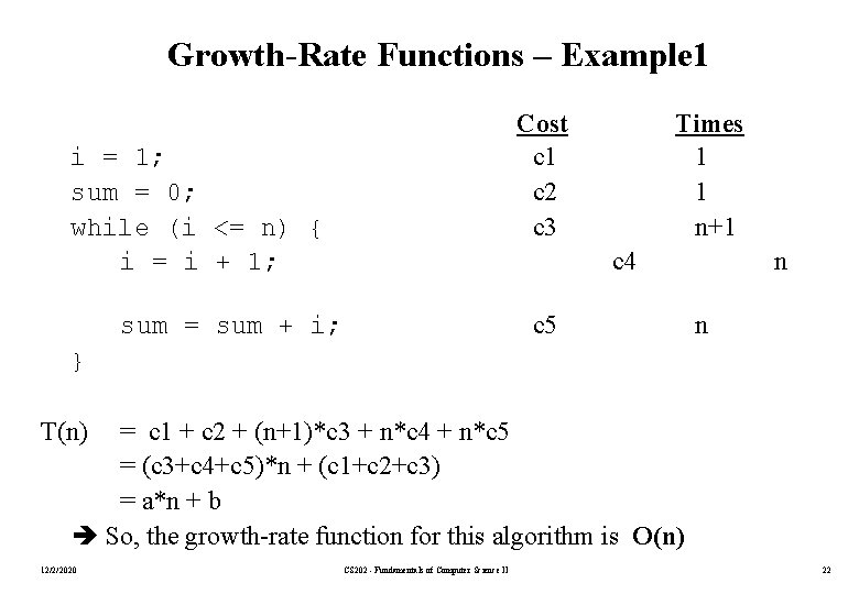
The Execution Time of Algorithms (cont. ) Example: Simple Loop Cost c 1 c 2 c 3 i = 1; sum = 0; while (i <= n) { i = i + 1; Times 1 1 n+1 c 4 c 5 sum = sum + i; n n } Total Cost = c 1 + c 2 + (n+1)*c 3 + n*c 4 + n*c 5 The time required for this algorithm is proportional to n 12/2/2020 CS 202 - Fundamentals of Computer Science II 7

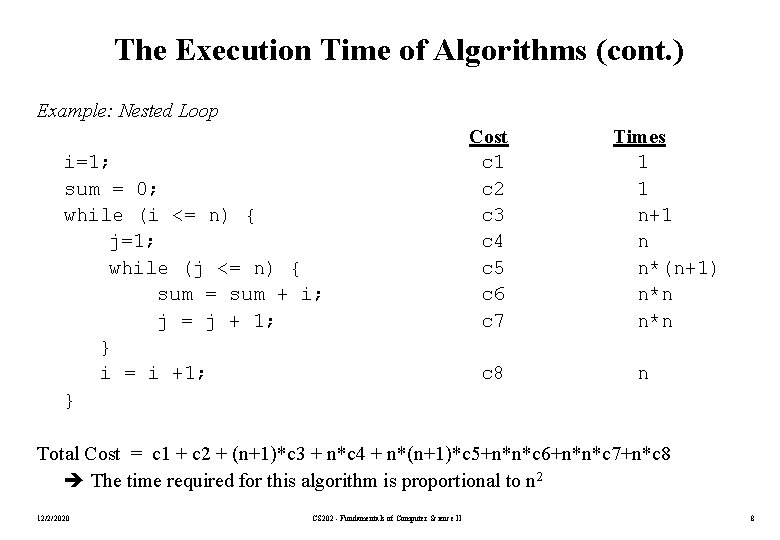
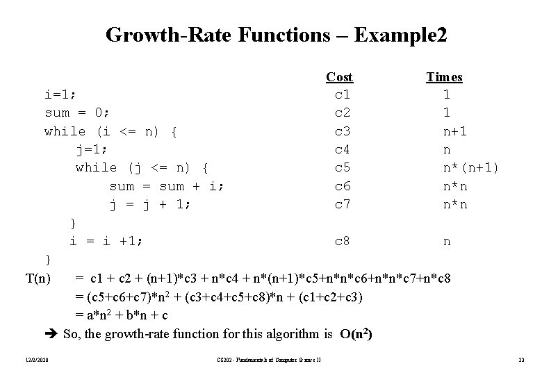
The Execution Time of Algorithms (cont. ) Example: Nested Loop i=1; sum = 0; while (i <= n) { j=1; while (j <= n) { sum = sum + i; j = j + 1; } i = i +1; } Cost c 1 c 2 c 3 c 4 c 5 c 6 c 7 c 8 Times 1 1 n+1 n n*(n+1) n*n n Total Cost = c 1 + c 2 + (n+1)*c 3 + n*c 4 + n*(n+1)*c 5+n*n*c 6+n*n*c 7+n*c 8 The time required for this algorithm is proportional to n 2 12/2/2020 CS 202 - Fundamentals of Computer Science II 8

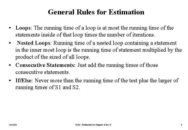
General Rules for Estimation • Loops: The running time of a loop is at most the running time of the statements inside of that loop times the number of iterations. • Nested Loops: Running time of a nested loop containing a statement in the inner most loop is the running time of statement multiplied by the product of the sized of all loops. • Consecutive Statements: Just add the running times of those consecutive statements. • If/Else: Never more than the running time of the test plus the larger of running times of S 1 and S 2. 12/2/2020 CS 202 - Fundamentals of Computer Science II 9

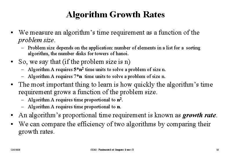
Algorithm Growth Rates • We measure an algorithm’s time requirement as a function of the problem size. – Problem size depends on the application: number of elements in a list for a sorting algorithm, the number disks for towers of hanoi. • So, we say that (if the problem size is n) – Algorithm A requires 5*n 2 time units to solve a problem of size n. – Algorithm A requires 7*n time units to solve a problem of size n. • The most important thing to learn is how quickly the algorithm’s time requirement grows a function of the problem size. – Algorithm A requires time proportional to n 2. – Algorithm A requires time proportional to n. • An algorithm’s proportional time requirement is known as growth rate. • We can compare the efficiency of two algorithms by comparing their growth rates. 12/2/2020 CS 202 - Fundamentals of Computer Science II 10

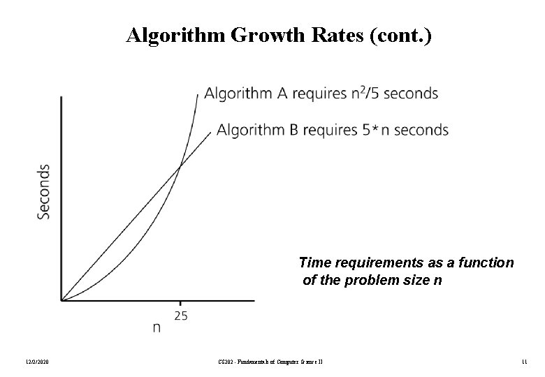
Algorithm Growth Rates (cont. ) Time requirements as a function of the problem size n 12/2/2020 CS 202 - Fundamentals of Computer Science II 11

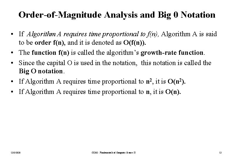
Order-of-Magnitude Analysis and Big 0 Notation • If Algorithm A requires time proportional to f(n), Algorithm A is said to be order f(n), and it is denoted as O(f(n)). • The function f(n) is called the algorithm’s growth-rate function. • Since the capital O is used in the notation, this notation is called the Big O notation. • If Algorithm A requires time proportional to n 2, it is O(n 2). • If Algorithm A requires time proportional to n, it is O(n). 12/2/2020 CS 202 - Fundamentals of Computer Science II 12

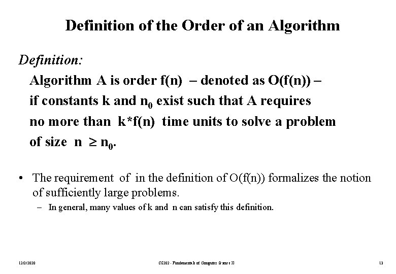
Definition of the Order of an Algorithm Definition: Algorithm A is order f(n) – denoted as O(f(n)) – if constants k and n 0 exist such that A requires no more than k*f(n) time units to solve a problem of size n n 0. • The requirement of in the definition of O(f(n)) formalizes the notion of sufficiently large problems. – In general, many values of k and n can satisfy this definition. 12/2/2020 CS 202 - Fundamentals of Computer Science II 13

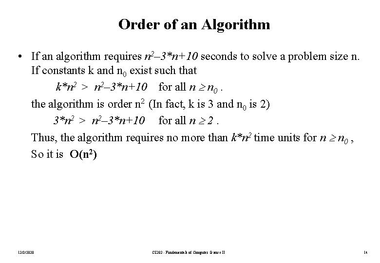
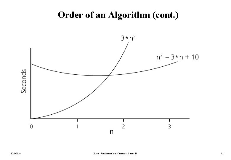
Order of an Algorithm • If an algorithm requires n 2– 3*n+10 seconds to solve a problem size n. If constants k and n 0 exist such that k*n 2 > n 2– 3*n+10 for all n n 0. the algorithm is order n 2 (In fact, k is 3 and n 0 is 2) 3*n 2 > n 2– 3*n+10 for all n 2. Thus, the algorithm requires no more than k*n 2 time units for n n 0 , So it is O(n 2) 12/2/2020 CS 202 - Fundamentals of Computer Science II 14

Order of an Algorithm (cont. ) 12/2/2020 CS 202 - Fundamentals of Computer Science II 15

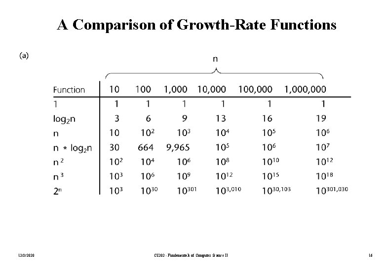
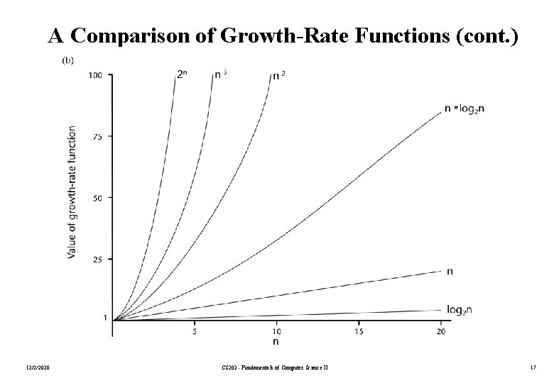
A Comparison of Growth-Rate Functions 12/2/2020 CS 202 - Fundamentals of Computer Science II 16

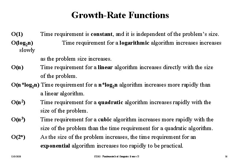
A Comparison of Growth-Rate Functions (cont. ) 12/2/2020 CS 202 - Fundamentals of Computer Science II 17

Growth-Rate Functions O(1) Time requirement is constant, and it is independent of the problem’s size. O(log 2 n) Time requirement for a logarithmic algorithm increases slowly as the problem size increases. O(n) Time requirement for a linear algorithm increases directly with the size of the problem. O(n*log 2 n) Time requirement for a n*log 2 n algorithm increases more rapidly than a linear algorithm. O(n 2) Time requirement for a quadratic algorithm increases rapidly with the size of the problem. O(n 3) Time requirement for a cubic algorithm increases more rapidly with the size of the problem than the time requirement for a quadratic algorithm. O(2 n) As the size of the problem increases, the time requirement for an exponential algorithm increases too rapidly to be practical. 12/2/2020 CS 202 - Fundamentals of Computer Science II 18

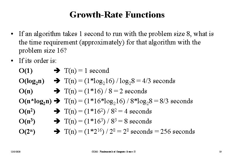
Growth-Rate Functions • If an algorithm takes 1 second to run with the problem size 8, what is the time requirement (approximately) for that algorithm with the problem size 16? • If its order is: O(1) T(n) = 1 second O(log 2 n) T(n) = (1*log 216) / log 28 = 4/3 seconds O(n) T(n) = (1*16) / 8 = 2 seconds O(n*log 2 n) T(n) = (1*16*log 216) / 8*log 28 = 8/3 seconds O(n 2) T(n) = (1*162) / 82 = 4 seconds O(n 3) T(n) = (1*163) / 83 = 8 seconds O(2 n) T(n) = (1*216) / 28 = 28 seconds = 256 seconds 12/2/2020 CS 202 - Fundamentals of Computer Science II 19

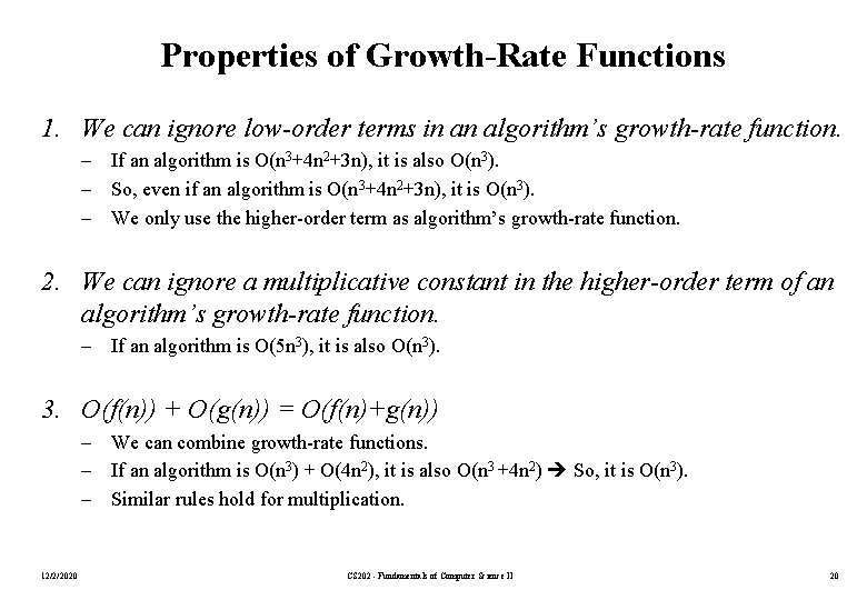
Properties of Growth-Rate Functions 1. We can ignore low-order terms in an algorithm’s growth-rate function. – If an algorithm is O(n 3+4 n 2+3 n), it is also O(n 3). – So, even if an algorithm is O(n 3+4 n 2+3 n), it is O(n 3). – We only use the higher-order term as algorithm’s growth-rate function. 2. We can ignore a multiplicative constant in the higher-order term of an algorithm’s growth-rate function. – If an algorithm is O(5 n 3), it is also O(n 3). 3. O(f(n)) + O(g(n)) = O(f(n)+g(n)) – We can combine growth-rate functions. – If an algorithm is O(n 3) + O(4 n 2), it is also O(n 3 +4 n 2) So, it is O(n 3). – Similar rules hold for multiplication. 12/2/2020 CS 202 - Fundamentals of Computer Science II 20

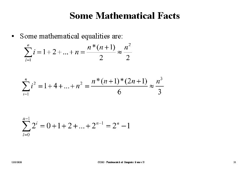
Some Mathematical Facts • Some mathematical equalities are: 12/2/2020 CS 202 - Fundamentals of Computer Science II 21

Growth-Rate Functions – Example 1 Cost c 1 c 2 c 3 i = 1; sum = 0; while (i <= n) { i = i + 1; Times 1 1 n+1 c 4 c 5 sum = sum + i; n n } T(n) = c 1 + c 2 + (n+1)*c 3 + n*c 4 + n*c 5 = (c 3+c 4+c 5)*n + (c 1+c 2+c 3) = a*n + b So, the growth-rate function for this algorithm is O(n) 12/2/2020 CS 202 - Fundamentals of Computer Science II 22

Growth-Rate Functions – Example 2 Cost c 1 c 2 c 3 c 4 c 5 c 6 c 7 Times 1 1 n+1 n n*(n+1) n*n i=1; sum = 0; while (i <= n) { j=1; while (j <= n) { sum = sum + i; j = j + 1; } i = i +1; c 8 n } T(n) = c 1 + c 2 + (n+1)*c 3 + n*c 4 + n*(n+1)*c 5+n*n*c 6+n*n*c 7+n*c 8 = (c 5+c 6+c 7)*n 2 + (c 3+c 4+c 5+c 8)*n + (c 1+c 2+c 3) = a*n 2 + b*n + c So, the growth-rate function for this algorithm is O(n 2) 12/2/2020 CS 202 - Fundamentals of Computer Science II 23

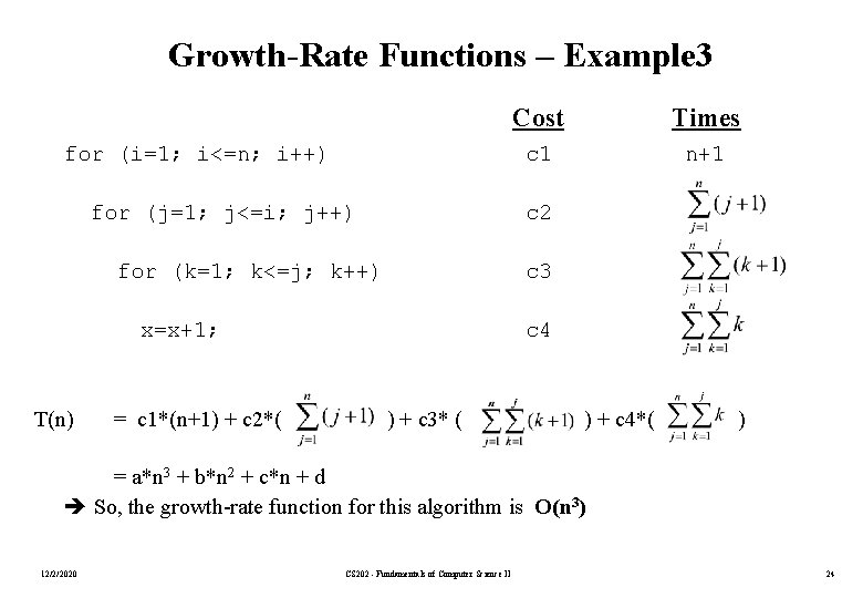
Growth-Rate Functions – Example 3 for (i=1; i<=n; i++) for (j=1; j<=i; j++) for (k=1; k<=j; k++) x=x+1; T(n) Cost Times c 1 n+1 c 2 c 3 c 4 = c 1*(n+1) + c 2*( ) + c 3* ( ) + c 4*( ) = a*n 3 + b*n 2 + c*n + d So, the growth-rate function for this algorithm is O(n 3) 12/2/2020 CS 202 - Fundamentals of Computer Science II 24

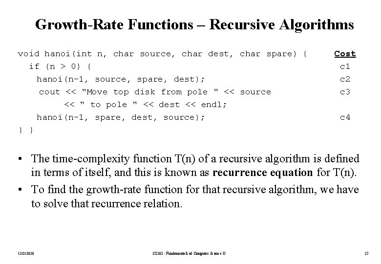
Growth-Rate Functions – Recursive Algorithms void hanoi(int n, char source, char dest, char spare) { if (n > 0) { hanoi(n-1, source, spare, dest); cout << "Move top disk from pole " << source << " to pole " << dest << endl; hanoi(n-1, spare, dest, source); } } Cost c 1 c 2 c 3 c 4 • The time-complexity function T(n) of a recursive algorithm is defined in terms of itself, and this is known as recurrence equation for T(n). • To find the growth-rate function for that recursive algorithm, we have to solve that recurrence relation. 12/2/2020 CS 202 - Fundamentals of Computer Science II 25

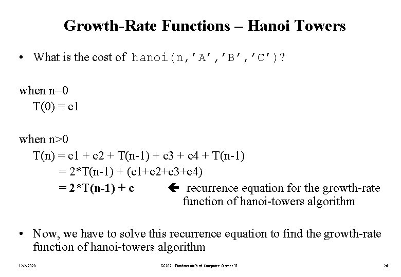
Growth-Rate Functions – Hanoi Towers • What is the cost of hanoi(n, ’A’, ’B’, ’C’)? when n=0 T(0) = c 1 when n>0 T(n) = c 1 + c 2 + T(n-1) + c 3 + c 4 + T(n-1) = 2*T(n-1) + (c 1+c 2+c 3+c 4) = 2*T(n-1) + c recurrence equation for the growth-rate function of hanoi-towers algorithm • Now, we have to solve this recurrence equation to find the growth-rate function of hanoi-towers algorithm 12/2/2020 CS 202 - Fundamentals of Computer Science II 26

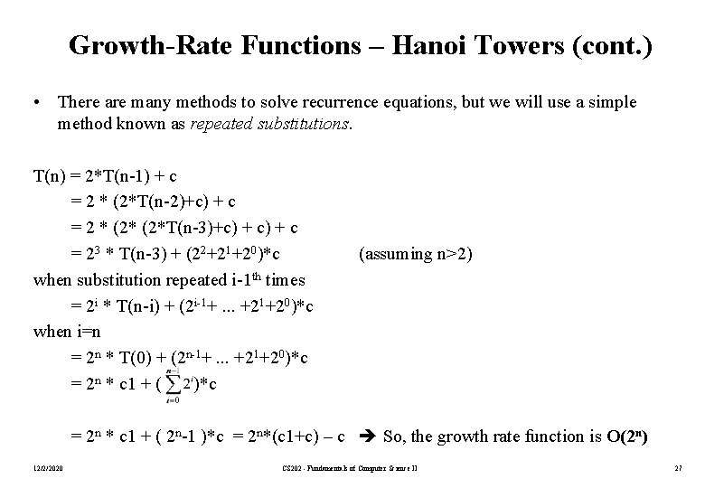
Growth-Rate Functions – Hanoi Towers (cont. ) • There are many methods to solve recurrence equations, but we will use a simple method known as repeated substitutions. T(n) = 2*T(n-1) + c = 2 * (2*T(n-2)+c) + c = 2 * (2*T(n-3)+c) + c = 23 * T(n-3) + (22+21+20)*c when substitution repeated i-1 th times = 2 i * T(n-i) + (2 i-1+. . . +21+20)*c when i=n = 2 n * T(0) + (2 n-1+. . . +21+20)*c = 2 n * c 1 + ( )*c (assuming n>2) = 2 n * c 1 + ( 2 n-1 )*c = 2 n*(c 1+c) – c So, the growth rate function is O(2 n) 12/2/2020 CS 202 - Fundamentals of Computer Science II 27

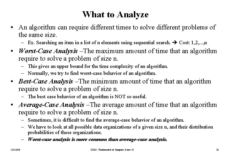
What to Analyze • An algorithm can require different times to solve different problems of the same size. – Ex. Searching an item in a list of n elements using sequential search. Cost: 1, 2, . . . , n • Worst-Case Analysis –The maximum amount of time that an algorithm require to solve a problem of size n. – This gives an upper bound for the time complexity of an algorithm. – Normally, we try to find worst-case behavior of an algorithm. • Best-Case Analysis –The minimum amount of time that an algorithm require to solve a problem of size n. – The best case behavior of an algorithm is NOT so useful. • Average-Case Analysis –The average amount of time that an algorithm require to solve a problem of size n. – Sometimes, it is difficult to find the average-case behavior of an algorithm. – We have to look at all possible data organizations of a given size n, and their distribution probabilities of these organizations. – Worst-case analysis is more common than average-case analysis. 12/2/2020 CS 202 - Fundamentals of Computer Science II 28

What is Important? • An array-based list retrieve operation is O(1), a linked-list-based list retrieve operation is O(n). • But insert and delete operations are much easier on a linked-list-based list implementation. When selecting an ADT’s implementations, we have to consider how frequently particular ADT operations occur in a given application. • If the problem size is always small, we can probably ignore an algorithm’s efficiency. – In this case, we should choose the simplest algorithm. 12/2/2020 CS 202 - Fundamentals of Computer Science II 29

What is Important? (cont. ) • We have to weigh the trade-offs between an algorithm’s time requirement and its memory requirements. • We have to compare algorithms for both style and efficiency. – The analysis should focus on gross differences in efficiency and not reward coding tricks that save small amount of time. – That is, there is no need for coding tricks if the gain is not too much. – Easily understandable program is also important. • Order-of-magnitude analysis focuses on large problems. 12/2/2020 CS 202 - Fundamentals of Computer Science II 30

Sequential Search int sequential. Search(const int a[], int item, int n){ for (int i = 0; i < n && a[i]!= item; i++); if (i == n) return – 1; return i; } Unsuccessful Search: O(n) Successful Search: Best-Case: item is in the first location of the array O(1) Worst-Case: item is in the last location of the array O(n) Average-Case: The number of key comparisons 1, 2, . . . , n O(n) 12/2/2020 CS 202 - Fundamentals of Computer Science II 31

Binary Search int binary. Search(int a[], int size, int x) { int low =0; int high = size – 1; int mid; // mid will be the index of // target when it’s found. while (low <= high) { mid = (low + high)/2; if (a[mid] < x) low = mid + 1; else if (a[mid] > x) high = mid – 1; else return mid; } return – 1; } 12/2/2020 CS 202 - Fundamentals of Computer Science II 32

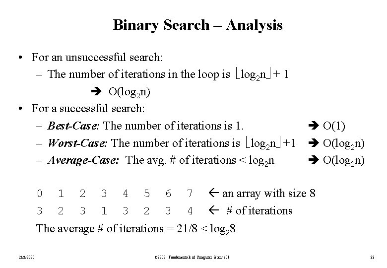
Binary Search – Analysis • For an unsuccessful search: – The number of iterations in the loop is log 2 n + 1 O(log 2 n) • For a successful search: – Best-Case: The number of iterations is 1. O(1) – Worst-Case: The number of iterations is log 2 n +1 O(log 2 n) – Average-Case: The avg. # of iterations < log 2 n O(log 2 n) 0 3 1 2 2 3 3 1 4 3 5 2 6 3 7 4 an array with size 8 # of iterations The average # of iterations = 21/8 < log 28 12/2/2020 CS 202 - Fundamentals of Computer Science II 33

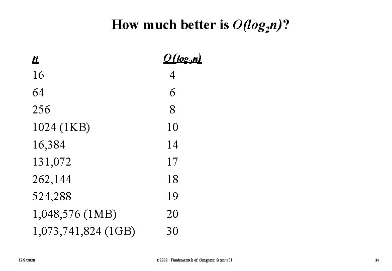
How much better is O(log 2 n)? n 16 64 256 1024 (1 KB) 16, 384 131, 072 262, 144 524, 288 1, 048, 576 (1 MB) 1, 073, 741, 824 (1 GB) 12/2/2020 O(log 2 n) 4 6 8 10 14 17 18 19 20 30 CS 202 - Fundamentals of Computer Science II 34

Binary Search – Analysis (cont. ) • Binary search is more efficient than sequential search. • Binary search algorithm is the best searching algorithm which uses key comparisons • Binary search requires a sorted list of items 12/2/2020 CS 202 - Fundamentals of Computer Science II 35

Sorting • Sorting is a process that organizes a collection of data into either ascending or descending order. • An internal sort requires that the collection of data fit entirely in the computer’s main memory. • We can use an external sort when the collection of data cannot fit in the computer’s main memory all at once but must reside in secondary storage such as on a disk. • We will analyze only internal sorting algorithms. • Any significant amount of computer output is generally arranged in some sorted order so that it can be interpreted. • Sorting also has indirect uses. An initial sort of the data can significantly enhance the performance of an algorithm. • Majority of programming projects use a sort somewhere, and in many cases, the sorting cost determines the running time. • A comparison-based sorting algorithm makes ordering decisions only on the basis of comparisons. 12/2/2020 CS 202 - Fundamentals of Computer Science II 36

Sorting Algorithms • There are many sorting algorithms, such as: – Selection Sort – Insertion Sort – Bubble Sort – Merge Sort – Quick Sort • First three sorting algorithms are not so efficient, but last two are efficient sorting algorithms. 12/2/2020 CS 202 - Fundamentals of Computer Science II 37

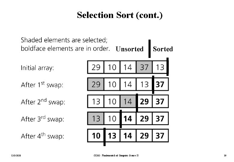
Selection Sort • The list is divided into two sublists, sorted and unsorted, which are divided by an imaginary wall. • We find the biggest element from the unsorted sublist and swap it with the element at the end of the unsorted data. • After each selection and swapping, the imaginary wall between the two sublists move one element back, increasing the number of sorted elements and decreasing the number of unsorted ones. • Each time we move one element from the unsorted sublist to the sorted sublist, we say that we have completed a sort pass. • A list of n elements requires n-1 passes to completely rearrange the data. 12/2/2020 CS 202 - Fundamentals of Computer Science II 38

Selection Sort (cont. ) Unsorted 12/2/2020 CS 202 - Fundamentals of Computer Science II Sorted 39

Selection Sort (cont. ) typedef type-of-array-item Data. Type; void selection. Sort(Data. Type the. Array[], int n) { for (int last = n-1; last >= 1; --last) { int largest = index. Of. Largest(the. Array, last+1); swap(the. Array[largest], the. Array[last]); } } 12/2/2020 CS 202 - Fundamentals of Computer Science II 40

Selection Sort (cont. ) int index. Of. Largest(const Data. Type the. Array[], int size) { int index. So. Far = 0; for(int current. Index=1; current. Index<size; ++current. Index) { if (the. Array[current. Index] > the. Array[index. So. Far]) index. So. Far = current. Index; } return index. So. Far; } ----------------------------void swap(Data. Type &x, Data. Type &y) { Data. Type temp = x; x = y; y = temp; } 12/2/2020 CS 202 - Fundamentals of Computer Science II 41

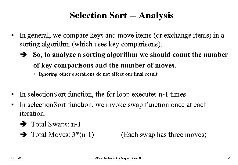
Selection Sort -- Analysis • In general, we compare keys and move items (or exchange items) in a sorting algorithm (which uses key comparisons). So, to analyze a sorting algorithm we should count the number of key comparisons and the number of moves. • Ignoring other operations do not affect our final result. • In selection. Sort function, the for loop executes n-1 times. • In selection. Sort function, we invoke swap function once at each iteration. Total Swaps: n-1 Total Moves: 3*(n-1) (Each swap has three moves) 12/2/2020 CS 202 - Fundamentals of Computer Science II 42

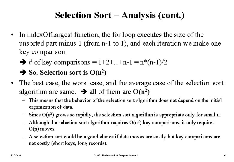
Selection Sort – Analysis (cont. ) • In index. Of. Largest function, the for loop executes the size of the unsorted part minus 1 (from n-1 to 1), and each iteration we make one key comparison. # of key comparisons = 1+2+. . . +n-1 = n*(n-1)/2 So, Selection sort is O(n 2) • The best case, the worst case, and the average case of the selection sort algorithm are same. all of them are O(n 2) – This means that the behavior of the selection sort algorithm does not depend on the initial organization of data. – Since O(n 2) grows so rapidly, the selection sort algorithm is appropriate only for small n. – Although the selection sort algorithm requires O(n 2) key comparisons, it only requires O(n) moves. – A selection sort could be a good choice if data moves are costly but key comparisons are not costly (short keys, long records). 12/2/2020 CS 202 - Fundamentals of Computer Science II 43

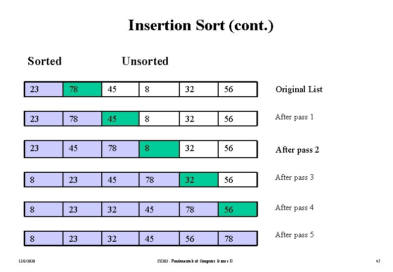
Insertion Sort • Insertion sort is a simple sorting algorithm that is appropriate for small inputs. – Most common sorting technique used by card players. • The list is divided into two parts: sorted and unsorted. • In each pass, the first element of the unsorted part is picked up, transferred to the sorted sublist, and inserted at the appropriate place. • A list of n elements will take at most n-1 passes to sort the data. 12/2/2020 CS 202 - Fundamentals of Computer Science II 44

Insertion Sort (cont. ) Sorted Unsorted 23 78 45 8 32 56 Original List 23 78 45 8 32 56 After pass 1 23 45 78 8 32 56 After pass 2 8 23 45 78 32 56 After pass 3 8 23 32 45 78 56 After pass 4 8 23 32 45 56 78 After pass 5 12/2/2020 CS 202 - Fundamentals of Computer Science II 45

Insertion Sort (cont. ) void insertion. Sort(Data. Type the. Array[], int n) { for (int unsorted = 1; unsorted < n; ++unsorted) { Data. Type next. Item = the. Array[unsorted]; int loc = unsorted; for (; (loc > 0) && (the. Array[loc-1] > next. Item); --loc) the. Array[loc] = the. Array[loc-1]; the. Array[loc] = next. Item; } } 12/2/2020 CS 202 - Fundamentals of Computer Science II 46

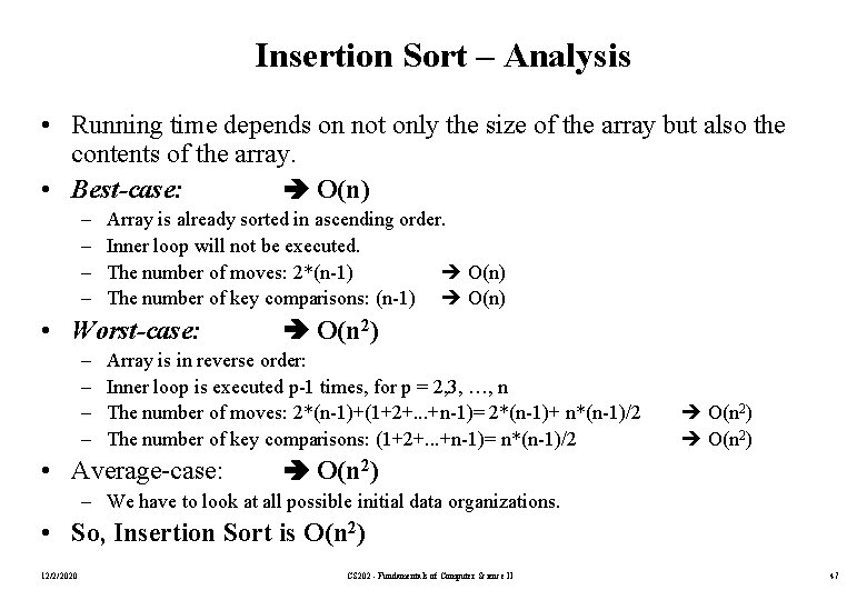
Insertion Sort – Analysis • Running time depends on not only the size of the array but also the contents of the array. • Best-case: O(n) – – Array is already sorted in ascending order. Inner loop will not be executed. The number of moves: 2*(n-1) O(n) The number of key comparisons: (n-1) O(n) • Worst-case: – – O(n 2) Array is in reverse order: Inner loop is executed p-1 times, for p = 2, 3, …, n The number of moves: 2*(n-1)+(1+2+. . . +n-1)= 2*(n-1)+ n*(n-1)/2 The number of key comparisons: (1+2+. . . +n-1)= n*(n-1)/2 • Average-case: O(n 2) – We have to look at all possible initial data organizations. • So, Insertion Sort is O(n 2) 12/2/2020 CS 202 - Fundamentals of Computer Science II 47

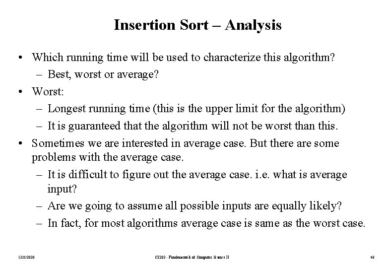
Insertion Sort – Analysis • Which running time will be used to characterize this algorithm? – Best, worst or average? • Worst: – Longest running time (this is the upper limit for the algorithm) – It is guaranteed that the algorithm will not be worst than this. • Sometimes we are interested in average case. But there are some problems with the average case. – It is difficult to figure out the average case. i. e. what is average input? – Are we going to assume all possible inputs are equally likely? – In fact, for most algorithms average case is same as the worst case. 12/2/2020 CS 202 - Fundamentals of Computer Science II 48

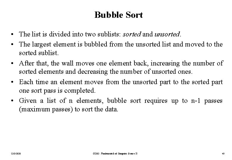
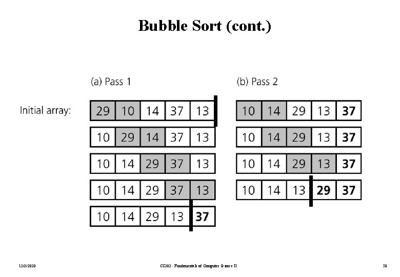
Bubble Sort • The list is divided into two sublists: sorted and unsorted. • The largest element is bubbled from the unsorted list and moved to the sorted sublist. • After that, the wall moves one element back, increasing the number of sorted elements and decreasing the number of unsorted ones. • Each time an element moves from the unsorted part to the sorted part one sort pass is completed. • Given a list of n elements, bubble sort requires up to n-1 passes (maximum passes) to sort the data. 12/2/2020 CS 202 - Fundamentals of Computer Science II 49

Bubble Sort (cont. ) 12/2/2020 CS 202 - Fundamentals of Computer Science II 50

Bubble Sort (cont. ) void bubble. Sort(Data. Type the. Array[], int n) { bool sorted = false; for (int pass = 1; (pass < n) && !sorted; ++pass) { sorted = true; for (int index = 0; index < n-pass; ++index) { int next. Index = index + 1; if (the. Array[index] > the. Array[next. Index]) { swap(the. Array[index], the. Array[next. Index]); sorted = false; // signal exchange } } 12/2/2020 CS 202 - Fundamentals of Computer Science II 51

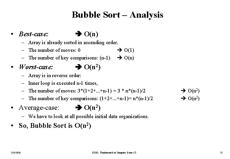
Bubble Sort – Analysis • Best-case: O(n) – Array is already sorted in ascending order. – The number of moves: 0 O(1) – The number of key comparisons: (n-1) O(n) • Worst-case: – – O(n 2) Array is in reverse order: Inner loop is executed n-1 times, The number of moves: 3*(1+2+. . . +n-1) = 3 * n*(n-1)/2 The number of key comparisons: (1+2+. . . +n-1)= n*(n-1)/2 • Average-case: O(n 2) – We have to look at all possible initial data organizations. • So, Bubble Sort is O(n 2) 12/2/2020 CS 202 - Fundamentals of Computer Science II 52

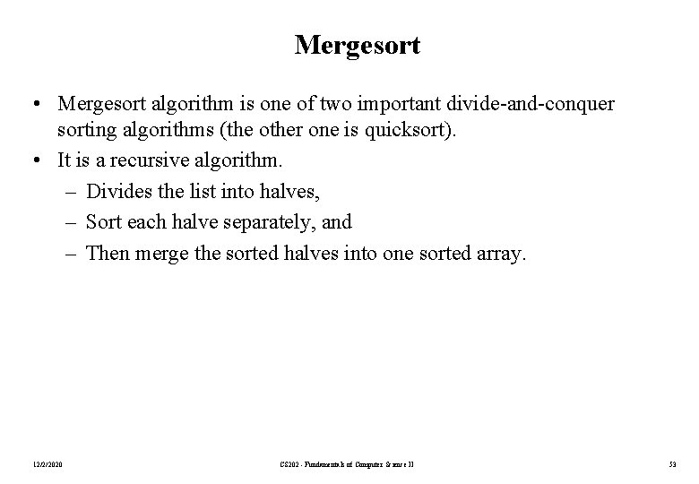
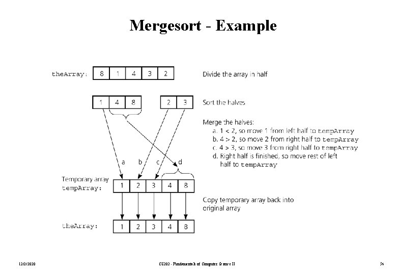
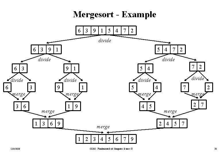
Mergesort • Mergesort algorithm is one of two important divide-and-conquer sorting algorithms (the other one is quicksort). • It is a recursive algorithm. – Divides the list into halves, – Sort each halve separately, and – Then merge the sorted halves into one sorted array. 12/2/2020 CS 202 - Fundamentals of Computer Science II 53

Mergesort - Example 12/2/2020 CS 202 - Fundamentals of Computer Science II 54

Merge const int MAX_SIZE = maximum-number-of-items-in-array; void merge(Data. Type the. Array[], int first, int mid, int last) { Data. Type temp. Array[MAX_SIZE]; // temporary array int first 1 = first; // beginning of first subarray int last 1 = mid; // end of first subarray int first 2 = mid + 1; // beginning of second subarray int last 2 = last; // end of second subarray int index = first 1; // next available location in temp. Array for ( ; (first 1 <= last 1) && (first 2 <= last 2); ++index) { if (the. Array[first 1] < the. Array[first 2]) { temp. Array[index] = the. Array[first 1]; ++first 1; } else { temp. Array[index] = the. Array[first 2]; ++first 2; } } 12/2/2020 CS 202 - Fundamentals of Computer Science II 55

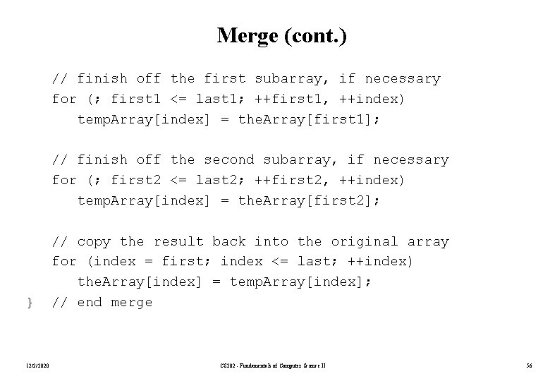
Merge (cont. ) // finish off the first subarray, if necessary for (; first 1 <= last 1; ++first 1, ++index) temp. Array[index] = the. Array[first 1]; // finish off the second subarray, if necessary for (; first 2 <= last 2; ++first 2, ++index) temp. Array[index] = the. Array[first 2]; } 12/2/2020 // copy the result back into the original array for (index = first; index <= last; ++index) the. Array[index] = temp. Array[index]; // end merge CS 202 - Fundamentals of Computer Science II 56

Mergesort void mergesort(Data. Type the. Array[], int first, int last) { if (first < last) { int mid = (first + last)/2; // index of midpoint mergesort(the. Array, first, mid); mergesort(the. Array, mid+1, last); // merge the two halves merge(the. Array, first, mid, last); } 12/2/2020 } // end mergesort CS 202 - Fundamentals of Computer Science II 57

Mergesort - Example 6 3 9 1 5 4 7 2 divide divide 6 3 9 1 5 4 7 2 merge 3 6 1 9 4 5 2 7 merge 1 3 6 9 merge 2 4 5 7 1 2 3 4 5 6 7 9 12/2/2020 CS 202 - Fundamentals of Computer Science II 58

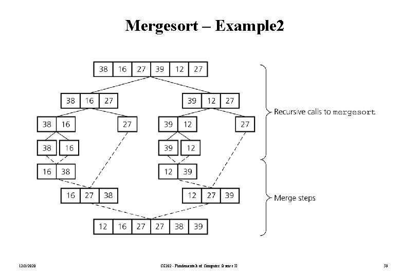
Mergesort – Example 2 12/2/2020 CS 202 - Fundamentals of Computer Science II 59

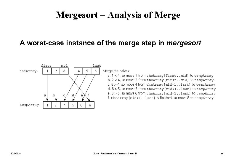
Mergesort – Analysis of Merge A worst-case instance of the merge step in mergesort 12/2/2020 CS 202 - Fundamentals of Computer Science II 60

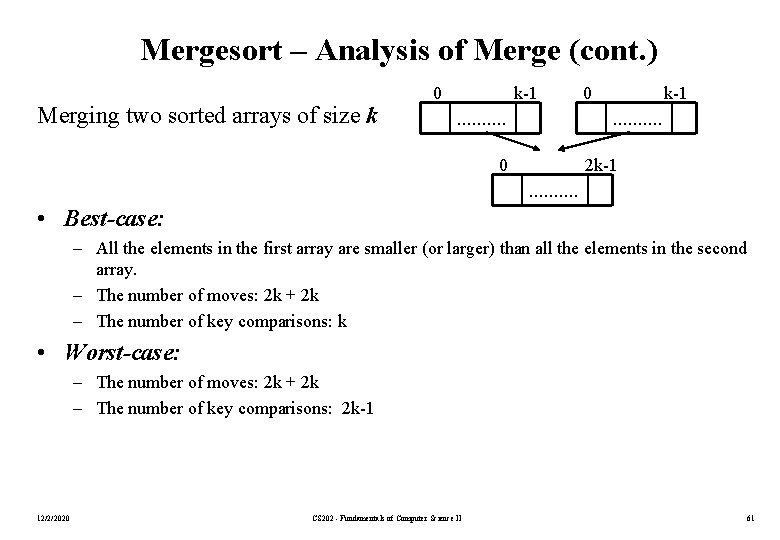
Mergesort – Analysis of Merge (cont. ) Merging two sorted arrays of size k 0 k-1 . . 0 2 k-1 . . • Best-case: – All the elements in the first array are smaller (or larger) than all the elements in the second array. – The number of moves: 2 k + 2 k – The number of key comparisons: k • Worst-case: – The number of moves: 2 k + 2 k – The number of key comparisons: 2 k-1 12/2/2020 CS 202 - Fundamentals of Computer Science II 61

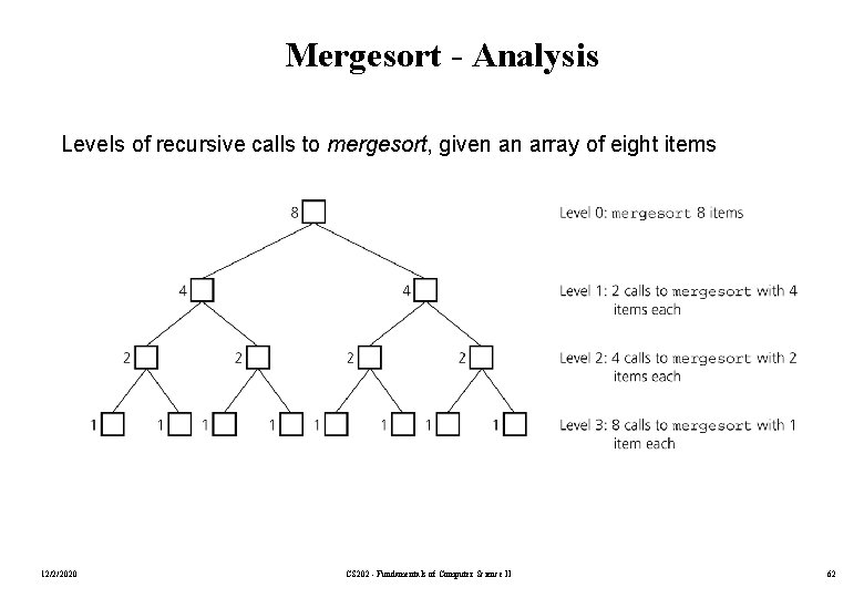
Mergesort - Analysis Levels of recursive calls to mergesort, given an array of eight items 12/2/2020 CS 202 - Fundamentals of Computer Science II 62

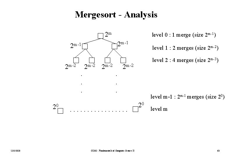
Mergesort - Analysis 2 m level 0 : 1 merge (size 2 m-1) 2 m-1 2 m-2 20 12/2/2020 . . . 2 m-2 . . . level 1 : 2 merges (size 2 m-2) level 2 : 4 merges (size 2 m-3) 2 m-2 . . . . CS 202 - Fundamentals of Computer Science II level m-1 : 2 m-1 merges (size 20) 20 level m 63

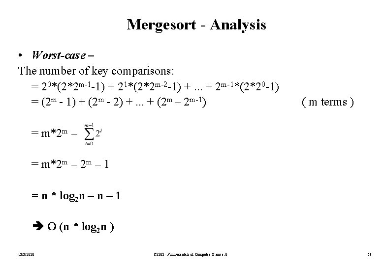
Mergesort - Analysis • Worst-case – The number of key comparisons: = 20*(2*2 m-1 -1) + 21*(2*2 m-2 -1) +. . . + 2 m-1*(2*20 -1) = (2 m - 1) + (2 m - 2) +. . . + (2 m – 2 m-1) ( m terms ) = m*2 m – 1 = n * log 2 n – 1 O (n * log 2 n ) 12/2/2020 CS 202 - Fundamentals of Computer Science II 64

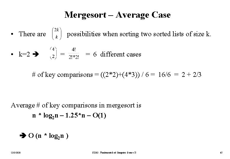
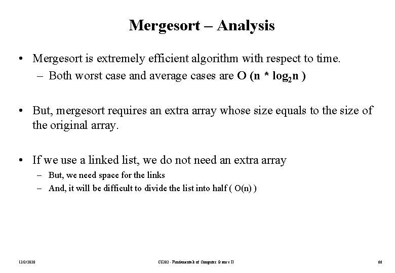
Mergesort – Average Case • There are possibilities when sorting two sorted lists of size k. • k=2 = = 6 different cases # of key comparisons = ((2*2)+(4*3)) / 6 = 16/6 = 2 + 2/3 Average # of key comparisons in mergesort is n * log 2 n – 1. 25*n – O(1) O (n * log 2 n ) 12/2/2020 CS 202 - Fundamentals of Computer Science II 65

Mergesort – Analysis • Mergesort is extremely efficient algorithm with respect to time. – Both worst case and average cases are O (n * log 2 n ) • But, mergesort requires an extra array whose size equals to the size of the original array. • If we use a linked list, we do not need an extra array – But, we need space for the links – And, it will be difficult to divide the list into half ( O(n) ) 12/2/2020 CS 202 - Fundamentals of Computer Science II 66

Quicksort • • • 12/2/2020 Like mergesort, Quicksort is also based on the divide-and-conquer paradigm. But it uses this technique in a somewhat opposite manner, as all the hard work is done before the recursive calls. It works 1. First, it partitions an array into two parts, 2. Then, it sorts the parts independently, 3. Finally, it combines the sorted subsequences by a simple concatenation. CS 202 - Fundamentals of Computer Science II 67

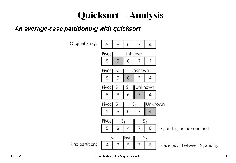
Quicksort (cont. ) The quick-sort algorithm consists of the following three steps: 1. Divide: Partition the list. – To partition the list, we first choose some element from the list for which we hope about half the elements will come before and half after. Call this element the pivot. – Then we partition the elements so that all those with values less than the pivot come in one sublist and all those with greater values come in another. 2. Recursion: Recursively sort the sublists separately. 3. Conquer: Put the sorted sublists together. 12/2/2020 CS 202 - Fundamentals of Computer Science II 68

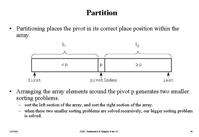
Partition • Partitioning places the pivot in its correct place position within the array. • Arranging the array elements around the pivot p generates two smaller sorting problems. – sort the left section of the array, and sort the right section of the array. – when these two smaller sorting problems are solved recursively, our bigger sorting problem is solved. 12/2/2020 CS 202 - Fundamentals of Computer Science II 69

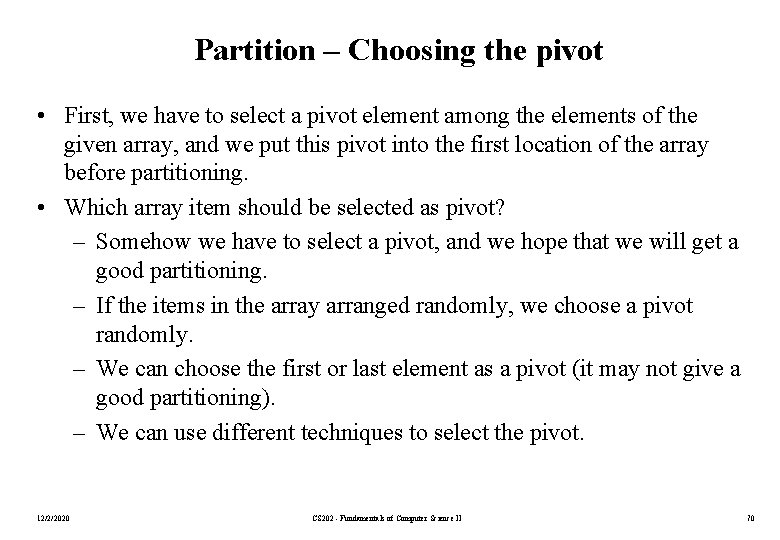
Partition – Choosing the pivot • First, we have to select a pivot element among the elements of the given array, and we put this pivot into the first location of the array before partitioning. • Which array item should be selected as pivot? – Somehow we have to select a pivot, and we hope that we will get a good partitioning. – If the items in the array arranged randomly, we choose a pivot randomly. – We can choose the first or last element as a pivot (it may not give a good partitioning). – We can use different techniques to select the pivot. 12/2/2020 CS 202 - Fundamentals of Computer Science II 70

Partition Function void partition(Data. Type the. Array[], int first, int last, int &pivot. Index) { // Partitions an array for quicksort. // Precondition: the. Array[first. . last] is an array; first <= last. // Postcondition: Partitions the. Array[first. . last] such that: // S 1 = the. Array[first. . pivot. Index-1] < pivot // the. Array[pivot. Index] == pivot // S 2 = the. Array[pivot. Index+1. . last] >= pivot // Calls: choose. Pivot and swap. // place pivot in the. Array[first] choose. Pivot(the. Array, first, last); Data. Type pivot = the. Array[first]; // copy pivot 12/2/2020 CS 202 - Fundamentals of Computer Science II 71

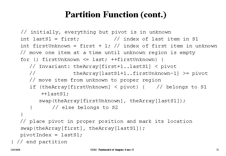
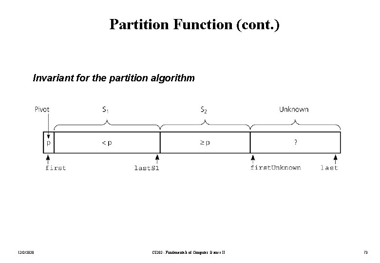
Partition Function (cont. ) // initially, everything but pivot is in unknown int last. S 1 = first; // index of last item in S 1 int first. Unknown = first + 1; // index of first item in unknown // move one item at a time until unknown region is empty for (; first. Unknown <= last; ++first. Unknown) { // Invariant: the. Array[first+1. . last. S 1] < pivot // the. Array[last. S 1+1. . first. Unknown-1] >= pivot // move item from unknown to proper region if (the. Array[first. Unknown] < pivot) { // belongs to S 1 ++last. S 1; swap(the. Array[first. Unknown], the. Array[last. S 1]); } // else belongs to S 2 } // place pivot in proper position and mark its location swap(the. Array[first], the. Array[last. S 1]); pivot. Index = last. S 1; } // end partition 12/2/2020 CS 202 - Fundamentals of Computer Science II 72

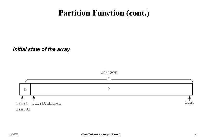
Partition Function (cont. ) Invariant for the partition algorithm 12/2/2020 CS 202 - Fundamentals of Computer Science II 73

Partition Function (cont. ) Initial state of the array 12/2/2020 CS 202 - Fundamentals of Computer Science II 74

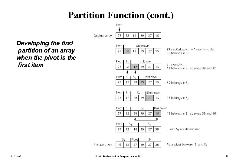
Partition Function (cont. ) Moving the. Array[first. Unknown] into S 1 by swapping it with the. Array[last. S 1+1] and by incrementing both last. S 1 and first. Unknown. 12/2/2020 CS 202 - Fundamentals of Computer Science II 75

Partition Function (cont. ) Moving the. Array[first. Unknown] into S 2 by incrementing first. Unknown. 12/2/2020 CS 202 - Fundamentals of Computer Science II 76

Partition Function (cont. ) Developing the first partition of an array when the pivot is the first item 12/2/2020 CS 202 - Fundamentals of Computer Science II 77

Quicksort Function void quicksort(Data. Type the. Array[], int first, int last) { // Sorts the items in an array into ascending order. // Precondition: the. Array[first. . last] is an array. // Postcondition: the. Array[first. . last] is sorted. // Calls: partition. int pivot. Index; if (first < last) { // create the partition: S 1, pivot, S 2 partition(the. Array, first, last, pivot. Index); // sort regions S 1 and S 2 quicksort(the. Array, first, pivot. Index-1); quicksort(the. Array, pivot. Index+1, last); } } 12/2/2020 CS 202 - Fundamentals of Computer Science II 78

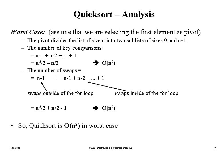
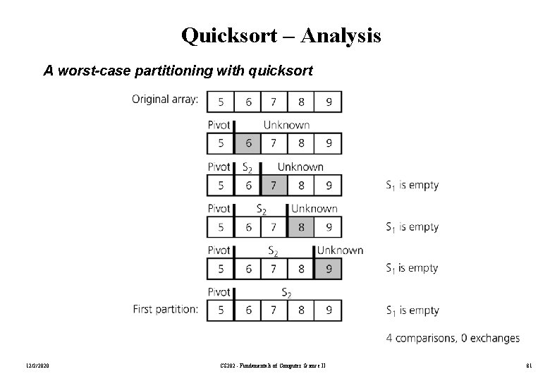
Quicksort – Analysis Worst Case: (assume that we are selecting the first element as pivot) – The pivot divides the list of size n into two sublists of sizes 0 and n-1. – The number of key comparisons = n-1 + n-2 +. . . + 1 = n 2/2 – n/2 O(n 2) – The number of swaps = = n-1 + n-2 +. . . + 1 swaps outside of the for loop = n 2/2 + n/2 - 1 swaps inside of the for loop O(n 2) • So, Quicksort is O(n 2) in worst case 12/2/2020 CS 202 - Fundamentals of Computer Science II 79

Quicksort – Analysis • Quicksort is O(n*log 2 n) in the best case and average case. • Quicksort is slow when the array is sorted and we choose the first element as the pivot. • Although the worst case behavior is not so good, and its average case behavior is much better than its worst case. – So, Quicksort is one of best sorting algorithms using key comparisons. • 12/2/2020 CS 202 - Fundamentals of Computer Science II 80

Quicksort – Analysis A worst-case partitioning with quicksort 12/2/2020 CS 202 - Fundamentals of Computer Science II 81

Quicksort – Analysis An average-case partitioning with quicksort 12/2/2020 CS 202 - Fundamentals of Computer Science II 82

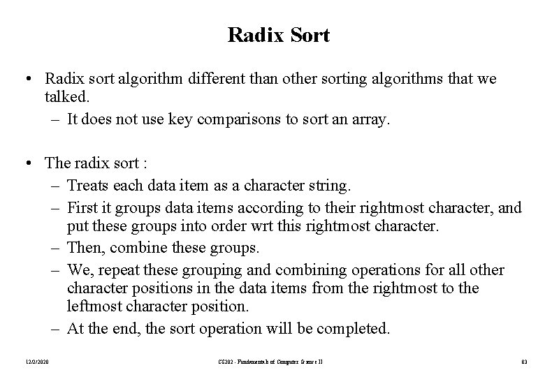
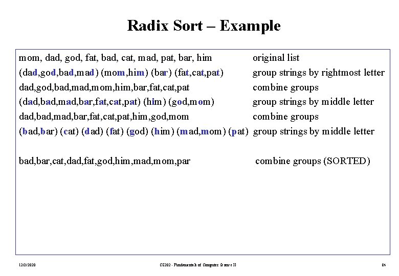
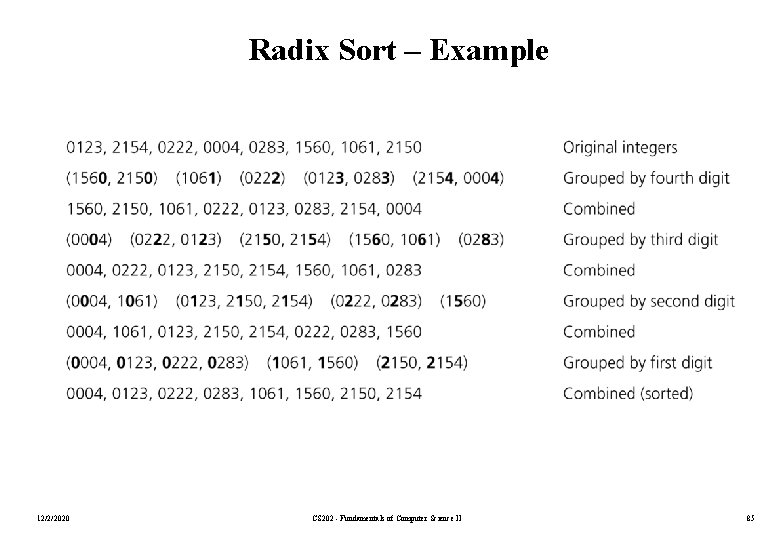
Radix Sort • Radix sort algorithm different than other sorting algorithms that we talked. – It does not use key comparisons to sort an array. • The radix sort : – Treats each data item as a character string. – First it groups data items according to their rightmost character, and put these groups into order wrt this rightmost character. – Then, combine these groups. – We, repeat these grouping and combining operations for all other character positions in the data items from the rightmost to the leftmost character position. – At the end, the sort operation will be completed. 12/2/2020 CS 202 - Fundamentals of Computer Science II 83

Radix Sort – Example mom, dad, god, fat, bad, cat, mad, pat, bar, him original list (dad, god, bad, mad) (mom, him) (bar) (fat, cat, pat) group strings by rightmost letter dad, god, bad, mom, him, bar, fat, cat, pat combine groups (dad, bad, mad, bar, fat, cat, pat) (him) (god, mom) group strings by middle letter dad, bad, mad, bar, fat, cat, pat, him, god, mom combine groups (bad, bar) (cat) (dad) (fat) (god) (him) (mad, mom) (pat) group strings by middle letter bad, bar, cat, dad, fat, god, him, mad, mom, par 12/2/2020 CS 202 - Fundamentals of Computer Science II combine groups (SORTED) 84

Radix Sort – Example 12/2/2020 CS 202 - Fundamentals of Computer Science II 85

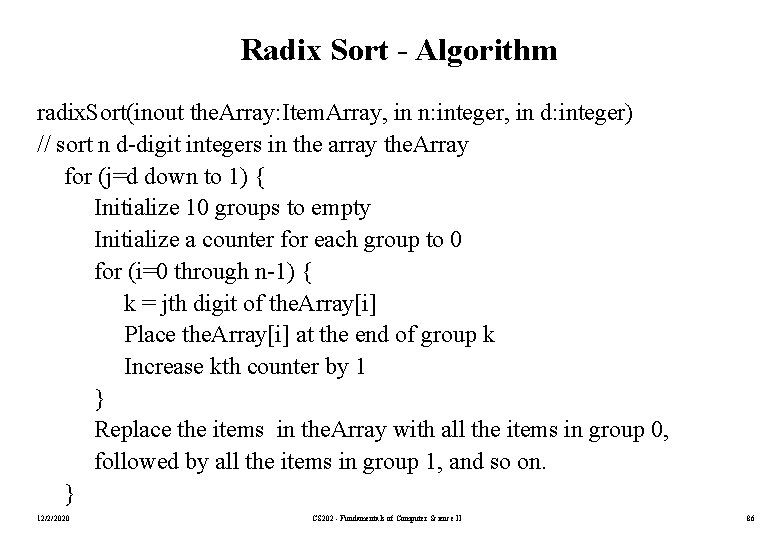
Radix Sort - Algorithm radix. Sort(inout the. Array: Item. Array, in n: integer, in d: integer) // sort n d-digit integers in the array the. Array for (j=d down to 1) { Initialize 10 groups to empty Initialize a counter for each group to 0 for (i=0 through n-1) { k = jth digit of the. Array[i] Place the. Array[i] at the end of group k Increase kth counter by 1 } Replace the items in the. Array with all the items in group 0, followed by all the items in group 1, and so on. } 12/2/2020 CS 202 - Fundamentals of Computer Science II 86

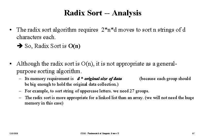
Radix Sort -- Analysis • The radix sort algorithm requires 2*n*d moves to sort n strings of d characters each. So, Radix Sort is O(n) • Although the radix sort is O(n), it is not appropriate as a generalpurpose sorting algorithm. – Its memory requirement is d * original size of data (because each group should be big enough to hold the original data collection. ) – For example, to sort string of uppercase letters. we need 27 groups. – The radix sort is more appropriate for a linked list than an array. (we will not need the huge memory in this case) 12/2/2020 CS 202 - Fundamentals of Computer Science II 87

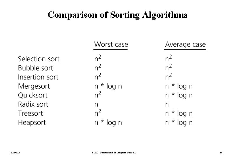
Comparison of Sorting Algorithms 12/2/2020 CS 202 - Fundamentals of Computer Science II 88