3 Related Paradoxes Including The Will Rogers Phenomenon

3 Related Paradoxes Including The Will Roger’s Phenomenon H. James Norton & George W. Divine norton 100@bellsouth. net Website: www. jimnortonphd. com

Paradoxes, by their very nature, can be interesting to students. These 3 paradoxes concerning IQs, gas mileage and cancer staging, are all related by a common thread. I use the first example when I teach introductory biostatistics to undergraduates and the 3 rd in a shortcourse for faculty and medical residents at the CMC.

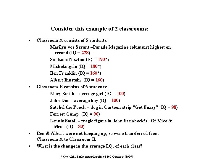
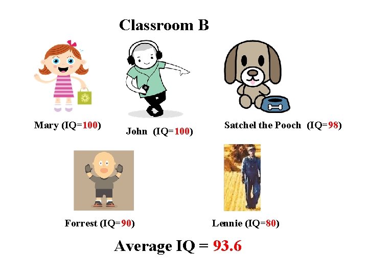
Consider this example of 2 classrooms: • • Classroom A consists of 5 students: Marilyn vos Savant –Parade Magazine columnist highest on record (IQ = 228) Sir Isaac Newton (IQ = 190*) Michelangelo (IQ = 180*) Ben Franklin (IQ = 160*) Albert Einstein (IQ = 160) Classroom B consists of 5 students: Mary Smith – average girl (IQ = 100) John Doe – average boy (IQ = 100) Satchel the Pooch – dog in Cartoon strip “Get Fuzzy” (IQ = 98) Forrest Gump (IQ = 90) Lennie Small – tragic figure in John Steinbeck’s “Of Mice & Men“ (IQ = 80) Ben & Albert were not keeping up, so were transferred from Classroom A to Classroom B. What is the change in the average I. Q. of each class? * Cox CM. , Early mental traits of 300 Geniuses (1926)

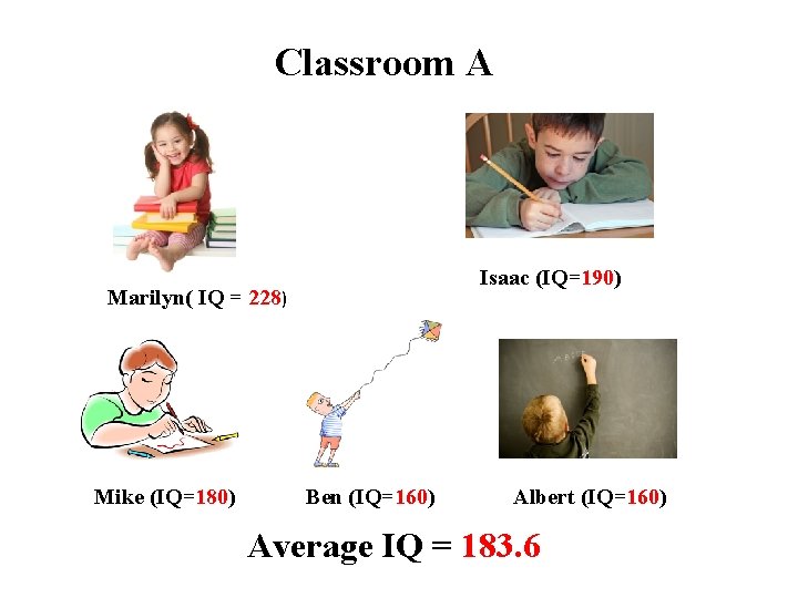
Classroom A Isaac (IQ=190) Marilyn( IQ = 228) Mike (IQ=180) Ben (IQ=160) Albert (IQ=160) Average IQ = 183. 6

Classroom B Mary (IQ=100) John (IQ=100) Forrest (IQ=90) Satchel the Pooch (IQ=98) Lennie (IQ=80) Average IQ = 93. 6

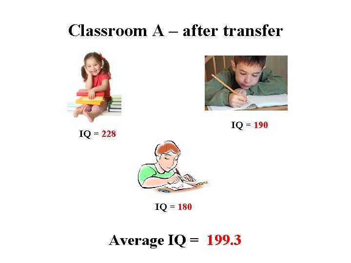
Classroom A – after transfer IQ = 190 IQ = 228 IQ = 180 Average IQ = 199. 3

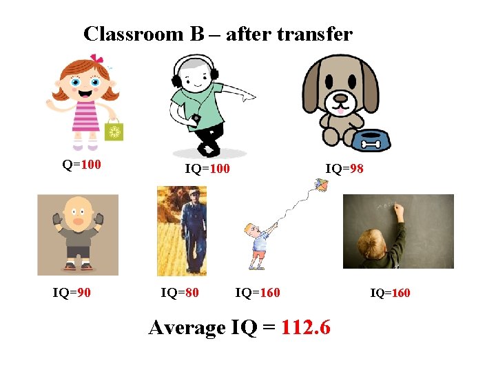
Classroom B – after transfer Q=100 IQ=90 IQ=100 IQ=80 IQ=98 IQ=160 Average IQ = 112. 6 IQ=160

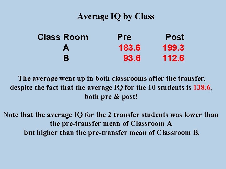
Average IQ by Class Room A B Pre 183. 6 93. 6 Post 199. 3 112. 6 The average went up in both classrooms after the transfer, despite the fact that the average IQ for the 10 students is 138. 6, both pre & post! Note that the average IQ for the 2 transfer students was lower than the pre-transfer mean of Classroom A but higher than the pre-transfer mean of Classroom B.

At Honest Abe’s Car & Truck Company. be part of we are proud to North Carolina’s Drive Green philosophy In the last year our fleet of cars has improved its gas mileage by 14. 8% & our trucks by 20. 7%!

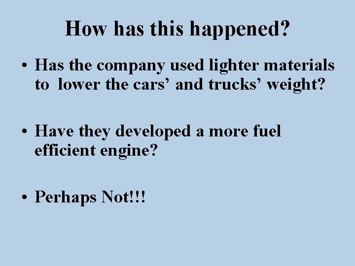
How has this happened? • Has the company used lighter materials to lower the cars’ and trucks’ weight? • Have they developed a more fuel efficient engine? • Perhaps Not!!!

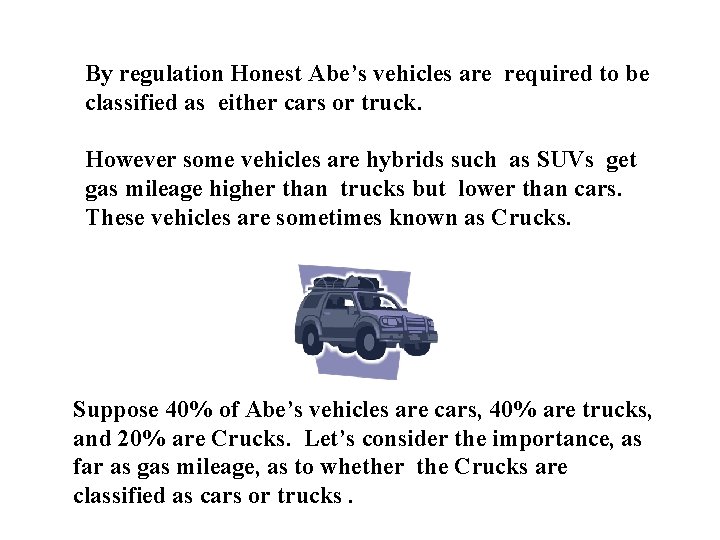
By regulation Honest Abe’s vehicles are required to be classified as either cars or truck. However some vehicles are hybrids such as SUVs get gas mileage higher than trucks but lower than cars. These vehicles are sometimes known as Crucks. Suppose 40% of Abe’s vehicles are cars, 40% are trucks, and 20% are Crucks. Let’s consider the importance, as far as gas mileage, as to whether the Crucks are classified as cars or trucks.

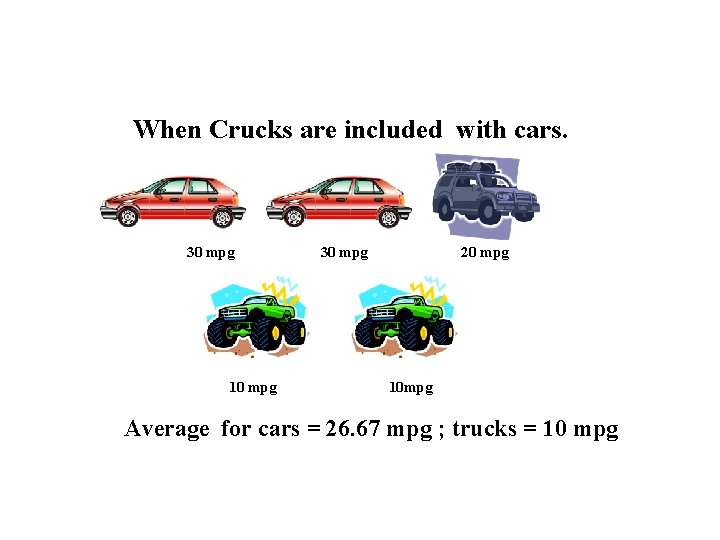
When Crucks are included with cars. 30 mpg 10 mpg 30 mpg 20 mpg 10 mpg Average for cars = 26. 67 mpg ; trucks = 10 mpg

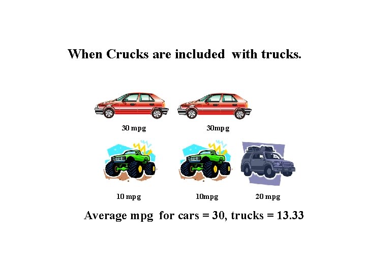
When Crucks are included with trucks. 30 mpg 10 mpg 30 mpg 10 mpg 20 mpg Average mpg for cars = 30, trucks = 13. 33

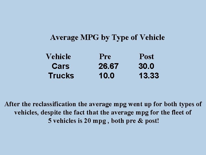
Average MPG by Type of Vehicle Cars Trucks Pre 26. 67 10. 0 Post 30. 0 13. 33 After the reclassification the average mpg went up for both types of vehicles, despite the fact that the average mpg for the fleet of 5 vehicles is 20 mpg , both pre & post!

Did Honest Abe (? ) improve his vehicles? No! He merely switched his Crucks from cars to trucks!!!

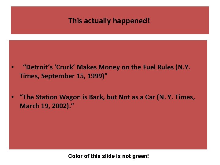
This actually happened! • “Detroit’s ‘Cruck’ Makes Money on the Fuel Rules (N. Y. Times, September 15, 1999)” • “The Station Wagon is Back, but Not as a Car (N. Y. Times, March 19, 2002). ” Color of this slide is not green!

http: //www. willrogers. org/

Will Rogers is the famous American Indian / cowboy / actor / raconteur known for saying: • “All I know is what I read in the papers” • “Everybody is ignorant. Only on different subjects. ” • “My ancestors didn’t come over on the Mayflower, but they met the boat”

In fact, Will Rogers has commented on statistics several times including: • “You can publish all the statistics and junk you want but I guess the whole country has been hit pretty hard. But I lay it to the Stock Market crash last fall” • “Statistics have proven there are 25 bathtubs sold to every Bible”

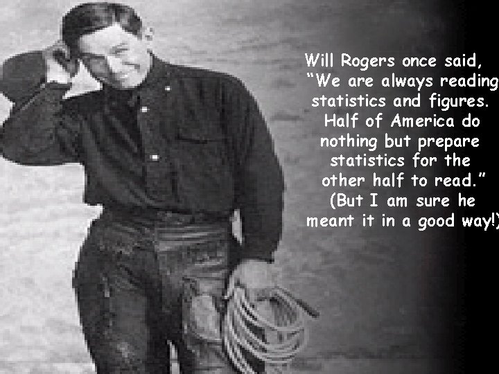
Will Rogers once said, “We are always reading statistics and figures. Half of America do nothing but prepare statistics for the other half to read. ” (But I am sure he meant it in a good way!)

He has also commented on life and death: • “Live your life so that whenever you lose, you’re ahead. ” • “If you live life right, death is a joke as far as fear is concerned. ”

A famous statistical paper contains Will Rogers’ name in the title: Feinstein AR, Sosin DM, Wells CK. The Will Rogers phenomenon: Stage migration and new diagnostic techniques as a source of misleading statistics for survival in cancer. N Engl J Med 1985 312: 25: 1604 -8. Much less famous: Norton HJ, Divine GW. The Will Rogers Effect The UMAP Journal 2007 28: 1: 75 -85.

Cancer patients are classified by stage • T – Tumor (size and depth of tumor) N – Nodes (has the cancer spread to the local lymph nodes) M – Metastases (has the cancer spread to distant organs) • These T, N, M components lead to an assignment of Stage 1 to 4 • More advanced disease is assigned a higher stage. (Stage 4 – tumor has metastasized)

A paradoxical situation can occur over time, where the overall death rate from a cancer may remain constant, but the death rate for every stage can down. This paradox is known as “The Will Rogers phenomenon. ”

Feinstein describes two sources of bias that may lead to the Will Rogers phenomenon • The Will Rogers phenomenon can make it appear that the survival rates for cancer are improving over time when, in fact, the overall survival rate remains completely constant. • The first bias is known as “lead-time” bias. This bias occurs when the cancer is diagnosed, for the average patient, at an earlier age than it might have been in a previous era due to improved screening techniques.

Biases leading to the Will Rogers phenomenon (continued) • A second bias is due to “stage migration. ” Patients diagnosed at a later time (e. g. , 2015) may be assigned to a higher stage than they would have at an earlier time point (e. g. , 1952) due to better assessment by improved medical technology. This phenomenon, that the more recent diagnosis, the more accurate the classification, is known as “stage migration. ”

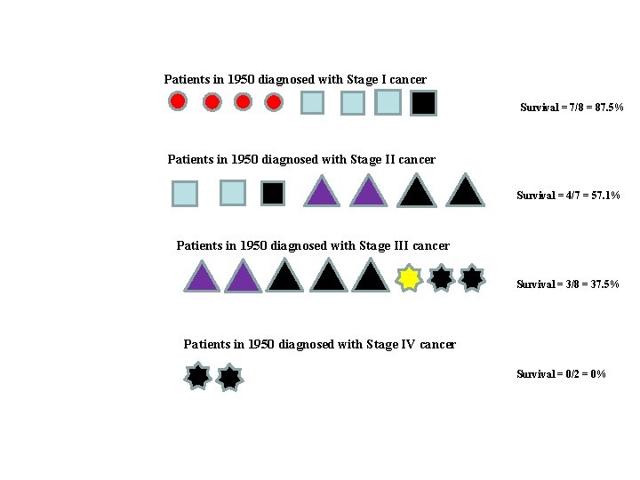
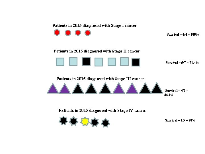
In our graphical presentation, Stage I in 1950 consists of two different symbols (circles and squares). This is because some of those patients, who are all classified as stage I in 1950, will be classified as stage II in 2015 due to improved technology. Similar situations apply to the 1950 classification of stage II and stage III patients.

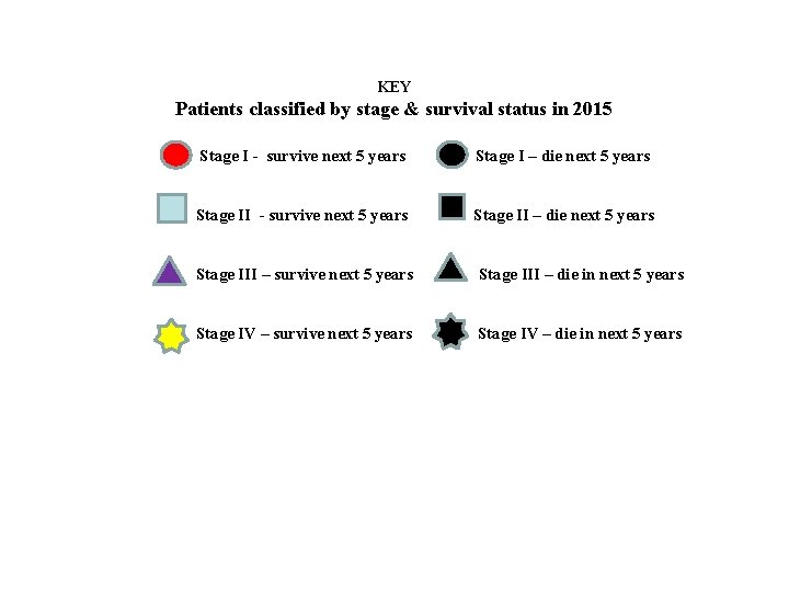
KEY Patients classified by stage & survival status in 2015 Stage I - survive next 5 years Stage I – die next 5 years Stage II - survive next 5 years Stage II – die next 5 years Stage III – survive next 5 years Stage III – die in next 5 years Stage IV – survive next 5 years Stage IV – die in next 5 years

Patients in 1950 diagnosed with Stage I cancer Survival = 7/8 = 87. 5% Patients in 1950 diagnosed with Stage II cancer Survival = 4/7 = 57. 1% Patients in 1950 diagnosed with Stage III cancer Survival = 3/8 = 37. 5% Patients in 1950 diagnosed with Stage IV cancer Survival = 0/2 = 0%

Patients in 2015 diagnosed with Stage I cancer Survival = 4/4 = 100% Patients in 2015 diagnosed with Stage II cancer Survival = 5/7 = 71. 4% Patients in 2015 diagnosed with Stage III cancer Survival = 4/9 = 44. 4% Patients in 2015 diagnosed with Stage IV cancer Survival = 1/5 = 20%

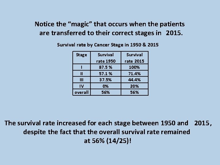
Notice the “magic” that occurs when the patients are transferred to their correct stages in 2015. Survival rate by Cancer Stage in 1950 & 2015 Stage I II IV overall Survival rate 1950 87. 5 % 57. 1 % 37. 5% 0% 56% Survival rate 2015 100% 71. 4% 44. 4% 20% 56% The survival rate increased for each stage between 1950 and 2015, despite the fact that the overall survival rate remained at 56% (14/25)!

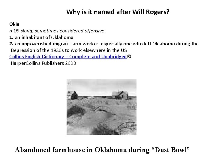
Why is it named after Will Rogers? Okie n US slang, sometimes considered offensive 1. an inhabitant of Oklahoma 2. an impoverished migrant farm worker, especially one who left Oklahoma during the Depression of the 1930 s to work elsewhere in the US Collins English Dictionary – Complete and Unabridged© Harper. Collins Publishers 2003 Abandoned farmhouse in Oklahoma during “Dust Bowl”

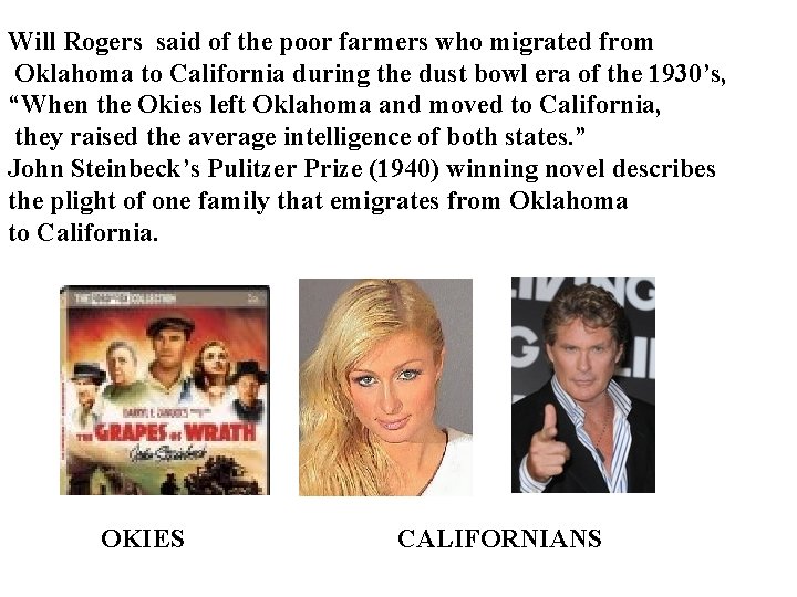
Will Rogers said of the poor farmers who migrated from Oklahoma to California during the dust bowl era of the 1930’s, “When the Okies left Oklahoma and moved to California, they raised the average intelligence of both states. ” John Steinbeck’s Pulitzer Prize (1940) winning novel describes the plight of one family that emigrates from Oklahoma to California. OKIES CALIFORNIANS

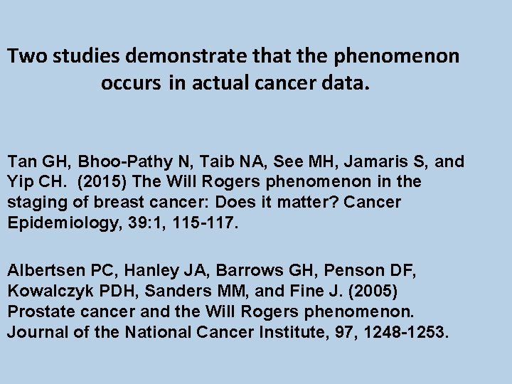
Two studies demonstrate that the phenomenon occurs in actual cancer data. Tan GH, Bhoo-Pathy N, Taib NA, See MH, Jamaris S, and Yip CH. (2015) The Will Rogers phenomenon in the staging of breast cancer: Does it matter? Cancer Epidemiology, 39: 1, 115 -117. Albertsen PC, Hanley JA, Barrows GH, Penson DF, Kowalczyk PDH, Sanders MM, and Fine J. (2005) Prostate cancer and the Will Rogers phenomenon. Journal of the National Cancer Institute, 97, 1248 -1253.

The American Joint Commission on Cancer (AJCC) updated staging for breast cancer in 2002 from the 5 th Edition to the 6 th Edition. Tan et al, demonstrated that this caused the Will Roger phenomenon to occur. 3127 cases of breast cancer were restaged from the 5 th Edition criteria to the 6 th Edition criteria. The percentage with late stage cancer increased from 27. 7% to 38. 1 %. Five-year survival improved in the women from 82. 9% to 86. 1% for stage II cancer and from 50. 6% to 59% for stage III.

Prostate cancer is graded and then a Gleason score is calculated. The Gleason score can range from 2 to 10. The higher the Gleason score, the worse is the prognosis. Slides from 1858 men who were diagnosed with prostate cancer in 1990 -1992 were blindly reread in 2002 -2004 (Albertsen et al). 55% of the cancers were upgraded to a higher Gleason score, while only 14% were downgraded. The survival rates increased for each of the Gleason score stratum.

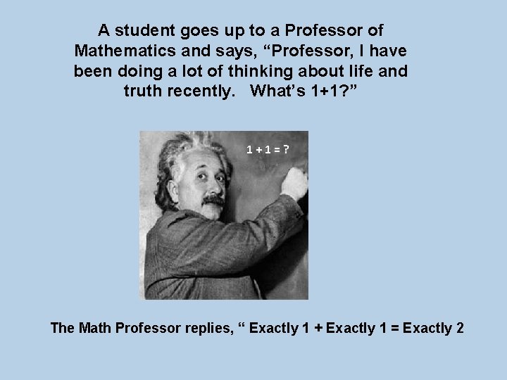
A student goes up to a Professor of Mathematics and says, “Professor, I have been doing a lot of thinking about life and truth recently. What’s 1+1? ” 1+1=? The Math Professor replies, “ Exactly 1 + Exactly 1 = Exactly 2

The student then goes up to a Professor of Computer Science and says, “Professor, I have been doing a lot of thinking about life and truth recently. What’s 1+1? ” The Computer Science Professor replies, “Approximately 1 + Approximately 1 = Approximately 2”

The student then goes up to his favorite teacher, a Professor of Statistics and says, “Professor, I have been doing a lot of thinking about life and truth recently. What’s 1+1? ” The Statistics Professor replies, “This is a deep and profound question. Please come into my office to discuss it. Then the Professor turns out the lights in the office and whispers into the student’s ear, “What do you want it to be? ”

Clearly the Statistics Professor violated the Ethical Guidelines for Statistical Practice and is no longer a member in good standing of ASA. He now works for “Honest Abe’s Car & Truck Company. ”

Conclusions: • Hopefully, the use of paradoxes & a little humor will improve the learning experience for the students. • Most students seem receptive to this style.

References 1. Feinstein AR, Sosin DM, and Wells CK. (1985) The Will Rogers phenomenon: Stage migration and new diagnostic techniques as a source of misleading statistics for survival in cancer. New England Journal of Medicine, 312: 25, 1604 -1608. 2. Norton HJ and Divine GW. (2007) The Will Rogers effect. The Journal of Undergraduate Mathematics and its Applications. 28: 1, 75 -85. 3. Tan GH, Bhoo-Pathy N, Taib NA, See MH, Jamaris S, and Yip CH. (2015) The Will Rogers phenomenon in the staging of breast cancer: Does it matter? Cancer Epidemiology, 39: 1, 115 -117. 4. Albertsen PC, Hanley JA, Barrows GH, Penson DF, Kowalczyk PDH, Sanders MM, and Fine J. (2005) Prostate cancer and the Will Rogers phenomenon. Journal of the National Cancer Institute, 97, 1248 -1253.