UNIT I Data Mining Concepts and Techniques Data

UNIT – I Data Mining: Concepts and Techniques & Data Preprocessing SNIST 1

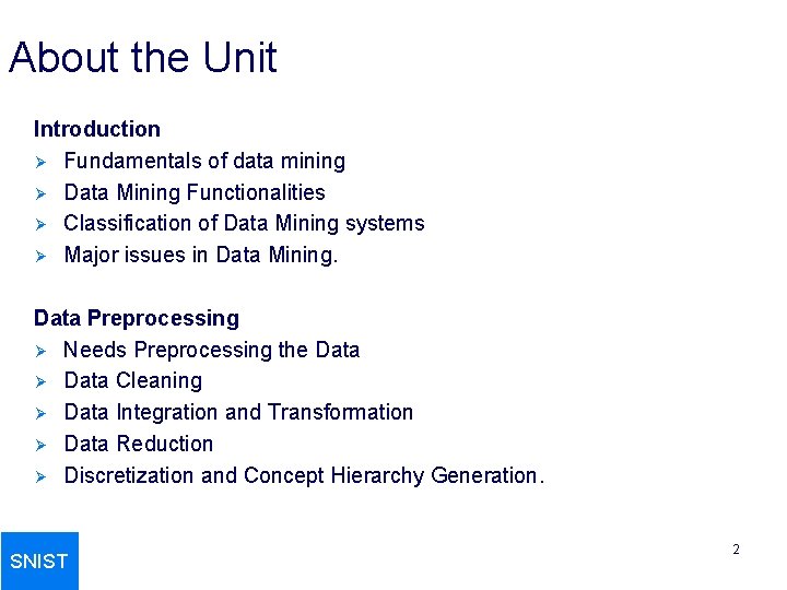
About the Unit Introduction Ø Fundamentals of data mining Ø Data Mining Functionalities Ø Classification of Data Mining systems Ø Major issues in Data Mining. Data Preprocessing Ø Needs Preprocessing the Data Ø Data Cleaning Ø Data Integration and Transformation Ø Data Reduction Ø Discretization and Concept Hierarchy Generation. SNIST 2

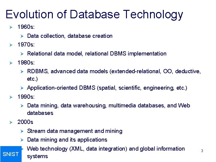
Evolution of Database Technology Ø 1960 s: Ø Ø 1970 s: Ø Ø Ø Relational data model, relational DBMS implementation 1980 s: Ø RDBMS, advanced data models (extended-relational, OO, deductive, etc. ) Ø Application-oriented DBMS (spatial, scientific, engineering, etc. ) 1990 s: Ø Ø Data collection, database creation Data mining, data warehousing, multimedia databases, and Web databases 2000 s SNIST Ø Stream data management and mining Ø Data mining and its applications Ø Web technology (XML, data integration) and global information systems 3

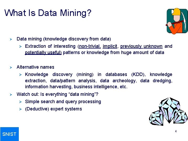
What Is Data Mining? Ø Data mining (knowledge discovery from data) Ø Ø Alternative names Ø Ø SNIST Extraction of interesting (non-trivial, implicit, previously unknown and potentially useful) patterns or knowledge from huge amount of data Knowledge discovery (mining) in databases (KDD), knowledge extraction, data/pattern analysis, data archeology, data dredging, information harvesting, business intelligence, etc. Watch out: Is everything “data mining”? Ø Simple search and query processing Ø (Deductive) expert systems 4

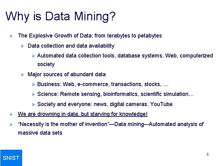
Why is Data Mining? Ø The Explosive Growth of Data: from terabytes to petabytes Ø Data collection and data availability Ø Automated data collection tools, database systems, Web, computerized society Ø Major sources of abundant data Ø Business: Web, e-commerce, transactions, stocks, … Ø Science: Remote sensing, bioinformatics, scientific simulation… Ø Society and everyone: news, digital cameras, You. Tube Ø We are drowning in data, but starving for knowledge! Ø “Necessity is the mother of invention”—Data mining—Automated analysis of massive data sets SNIST 5

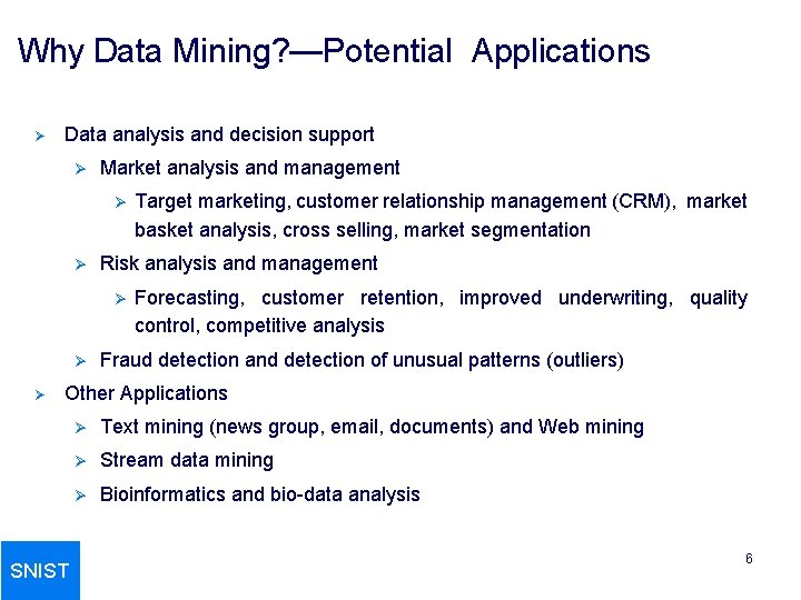
Why Data Mining? —Potential Applications Ø Data analysis and decision support Ø Market analysis and management Ø Ø Risk analysis and management Ø Ø Ø Target marketing, customer relationship management (CRM), market basket analysis, cross selling, market segmentation Forecasting, customer retention, improved underwriting, quality control, competitive analysis Fraud detection and detection of unusual patterns (outliers) Other Applications SNIST Ø Text mining (news group, email, documents) and Web mining Ø Stream data mining Ø Bioinformatics and bio-data analysis 6

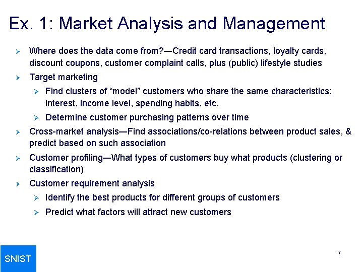
Ex. 1: Market Analysis and Management Ø Where does the data come from? —Credit card transactions, loyalty cards, discount coupons, customer complaint calls, plus (public) lifestyle studies Ø Target marketing Ø Find clusters of “model” customers who share the same characteristics: interest, income level, spending habits, etc. Ø Determine customer purchasing patterns over time Ø Cross-market analysis—Find associations/co-relations between product sales, & predict based on such association Ø Customer profiling—What types of customers buy what products (clustering or classification) Ø Customer requirement analysis SNIST Ø Identify the best products for different groups of customers Ø Predict what factors will attract new customers 7

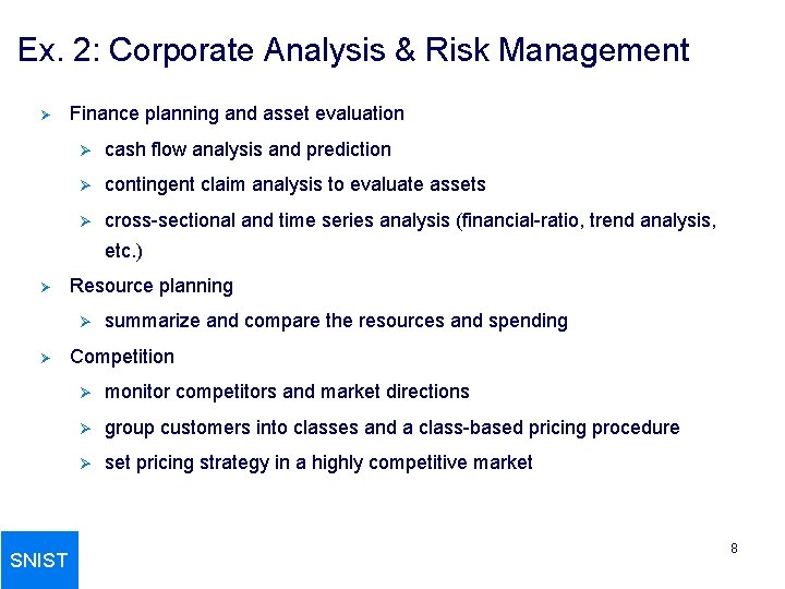
Ex. 2: Corporate Analysis & Risk Management Ø Finance planning and asset evaluation Ø cash flow analysis and prediction Ø contingent claim analysis to evaluate assets Ø cross-sectional and time series analysis (financial-ratio, trend analysis, etc. ) Ø Resource planning Ø Ø SNIST summarize and compare the resources and spending Competition Ø monitor competitors and market directions Ø group customers into classes and a class-based pricing procedure Ø set pricing strategy in a highly competitive market 8

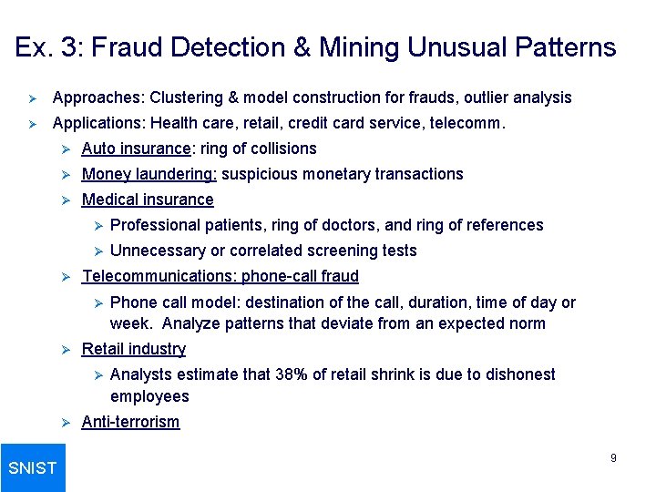
Ex. 3: Fraud Detection & Mining Unusual Patterns Ø Approaches: Clustering & model construction for frauds, outlier analysis Ø Applications: Health care, retail, credit card service, telecomm. Ø Auto insurance: ring of collisions Ø Money laundering: suspicious monetary transactions Ø Medical insurance Ø Ø Professional patients, ring of doctors, and ring of references Ø Unnecessary or correlated screening tests Telecommunications: phone-call fraud Ø Ø Retail industry Ø Ø SNIST Phone call model: destination of the call, duration, time of day or week. Analyze patterns that deviate from an expected norm Analysts estimate that 38% of retail shrink is due to dishonest employees Anti-terrorism 9

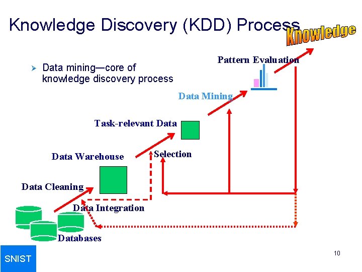
Knowledge Discovery (KDD) Process Ø Pattern Evaluation Data mining—core of knowledge discovery process Data Mining Task-relevant Data Warehouse Selection Data Cleaning Data Integration Databases SNIST 10

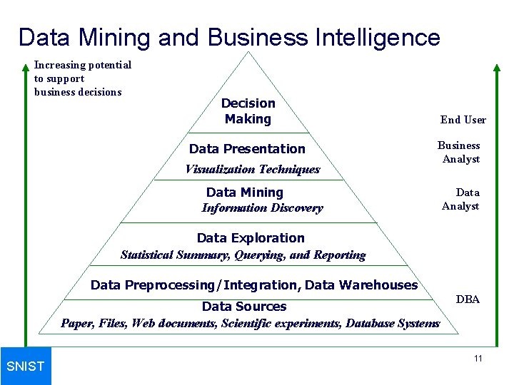
Data Mining and Business Intelligence Increasing potential to support business decisions Decision Making Data Presentation Visualization Techniques End User Business Analyst Data Mining Information Discovery Data Analyst Data Exploration Statistical Summary, Querying, and Reporting Data Preprocessing/Integration, Data Warehouses Data Sources Paper, Files, Web documents, Scientific experiments, Database Systems SNIST DBA 11

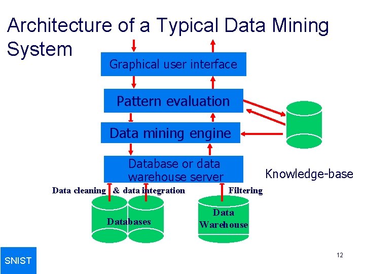
Architecture of a Typical Data Mining System Graphical user interface Pattern evaluation Data mining engine Database or data warehouse server Data cleaning & data integration Databases SNIST Knowledge-base Filtering Data Warehouse 12

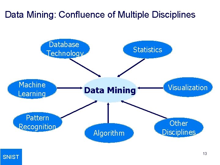
Data Mining: Confluence of Multiple Disciplines Database Technology Machine Learning Pattern Recognition SNIST Statistics Data Mining Algorithm Visualization Other Disciplines 13

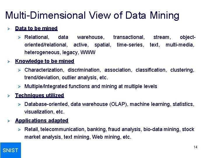
Multi-Dimensional View of Data Mining Ø Data to be mined Ø Ø Ø stream, objecttext, multi-media, Knowledge to be mined Ø Characterization, discrimination, association, classification, clustering, trend/deviation, outlier analysis, etc. Ø Multiple/integrated functions and mining at multiple levels Techniques utilized Ø Ø Relational, data warehouse, transactional, oriented/relational, active, spatial, time-series, heterogeneous, legacy, WWW Database-oriented, data warehouse (OLAP), machine learning, statistics, visualization, etc. Applications adapted Ø SNIST Retail, telecommunication, banking, fraud analysis, bio-data mining, stock market analysis, text mining, Web mining, etc. 14

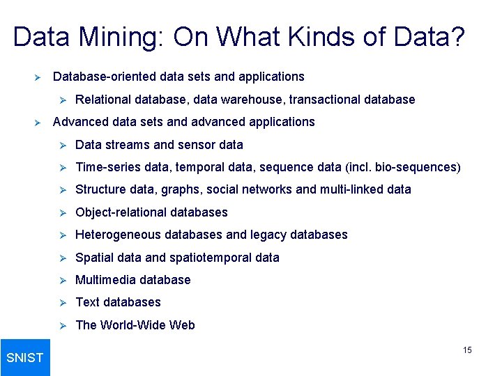
Data Mining: On What Kinds of Data? Ø Database-oriented data sets and applications Ø Ø SNIST Relational database, data warehouse, transactional database Advanced data sets and advanced applications Ø Data streams and sensor data Ø Time-series data, temporal data, sequence data (incl. bio-sequences) Ø Structure data, graphs, social networks and multi-linked data Ø Object-relational databases Ø Heterogeneous databases and legacy databases Ø Spatial data and spatiotemporal data Ø Multimedia database Ø Text databases Ø The World-Wide Web 15

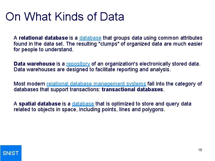
On What Kinds of Data A relational database is a database that groups data using common attributes found in the data set. The resulting "clumps" of organized data are much easier for people to understand. Data warehouse is a repository of an organization's electronically stored data. Data warehouses are designed to facilitate reporting and analysis. Most modern relational database management systems fall into the category of databases that support transactions: transactional databases. A spatial database is a database that is optimized to store and query data related to objects in space, including points, lines and polygons. SNIST 16

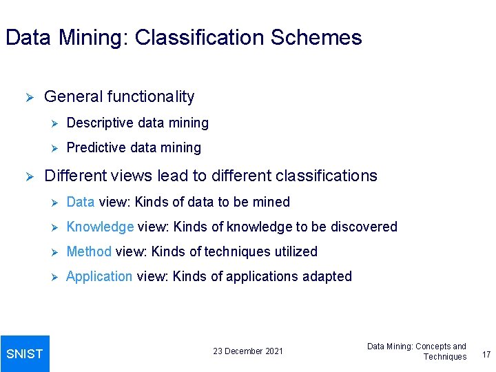
Data Mining: Classification Schemes Ø Ø SNIST General functionality Ø Descriptive data mining Ø Predictive data mining Different views lead to different classifications Ø Data view: Kinds of data to be mined Ø Knowledge view: Kinds of knowledge to be discovered Ø Method view: Kinds of techniques utilized Ø Application view: Kinds of applications adapted 23 December 2021 Data Mining: Concepts and Techniques 17

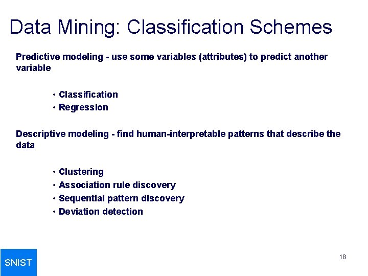
Data Mining: Classification Schemes Predictive modeling - use some variables (attributes) to predict another variable • Classification • Regression Descriptive modeling - find human-interpretable patterns that describe the data • Clustering • Association rule discovery • Sequential pattern discovery • Deviation detection SNIST 18

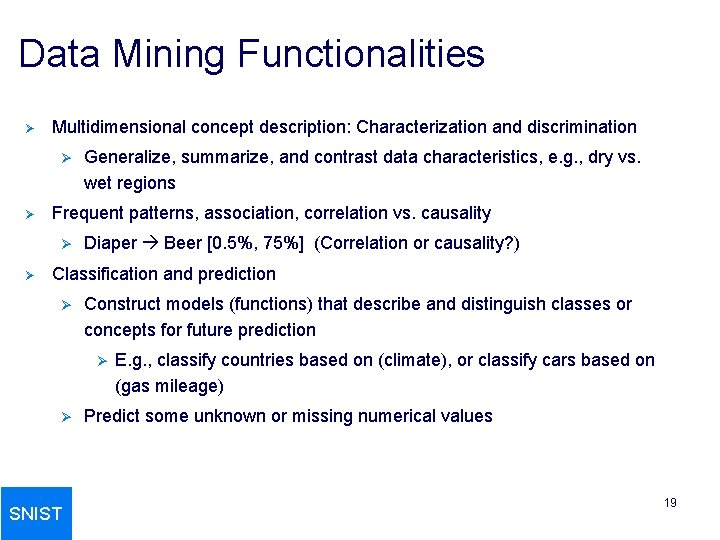
Data Mining Functionalities Ø Multidimensional concept description: Characterization and discrimination Ø Ø Frequent patterns, association, correlation vs. causality Ø Ø Generalize, summarize, and contrast data characteristics, e. g. , dry vs. wet regions Diaper Beer [0. 5%, 75%] (Correlation or causality? ) Classification and prediction Ø Construct models (functions) that describe and distinguish classes or concepts for future prediction Ø Ø SNIST E. g. , classify countries based on (climate), or classify cars based on (gas mileage) Predict some unknown or missing numerical values 19

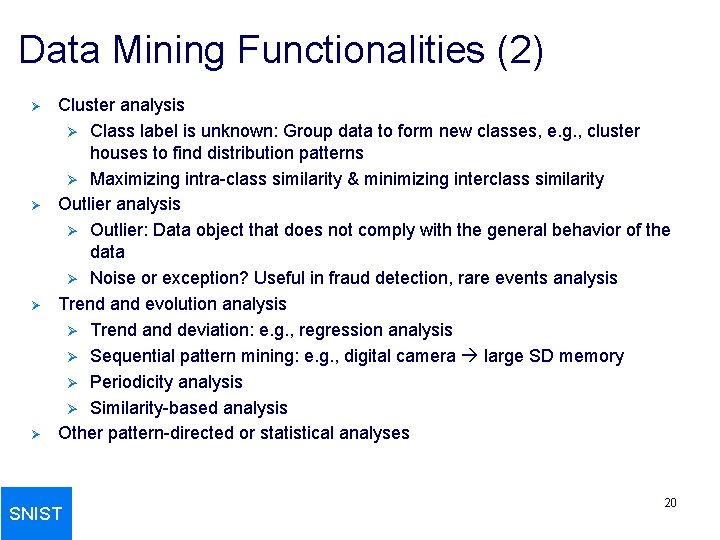
Data Mining Functionalities (2) Ø Ø Cluster analysis Ø Class label is unknown: Group data to form new classes, e. g. , cluster houses to find distribution patterns Ø Maximizing intra-class similarity & minimizing interclass similarity Outlier analysis Ø Outlier: Data object that does not comply with the general behavior of the data Ø Noise or exception? Useful in fraud detection, rare events analysis Trend and evolution analysis Ø Trend and deviation: e. g. , regression analysis Ø Sequential pattern mining: e. g. , digital camera large SD memory Ø Periodicity analysis Ø Similarity-based analysis Other pattern-directed or statistical analyses SNIST 20

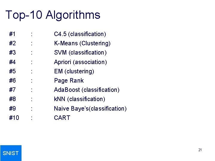
Top-10 Algorithms #1 : C 4. 5 (classification) #2 : K-Means (Clustering) #3 : SVM (classification) #4 : Apriori (association) #5 : EM (clustering) #6 : Page Rank #7 : Ada. Boost (classification) #8 : k. NN (classification) #9 : Naive Baye’s(classification) #10 : CART SNIST 21

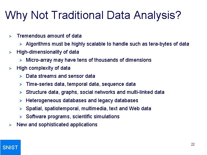
Why Not Traditional Data Analysis? Ø Tremendous amount of data Ø Ø High-dimensionality of data Ø Ø Ø Algorithms must be highly scalable to handle such as tera-bytes of data Micro-array may have tens of thousands of dimensions High complexity of data Ø Data streams and sensor data Ø Time-series data, temporal data, sequence data Ø Structure data, graphs, social networks and multi-linked data Ø Heterogeneous databases and legacy databases Ø Spatial, spatiotemporal, multimedia, text and Web data Ø Software programs, scientific simulations New and sophisticated applications SNIST 22

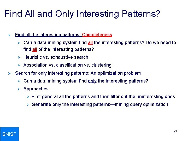
Find All and Only Interesting Patterns? Ø Ø Find all the interesting patterns: Completeness Ø Can a data mining system find all the interesting patterns? Do we need to find all of the interesting patterns? Ø Heuristic vs. exhaustive search Ø Association vs. classification vs. clustering Search for only interesting patterns: An optimization problem SNIST Ø Can a data mining system find only the interesting patterns? Ø Approaches Ø First general all the patterns and then filter out the uninteresting ones Ø Generate only the interesting patterns—mining query optimization 23

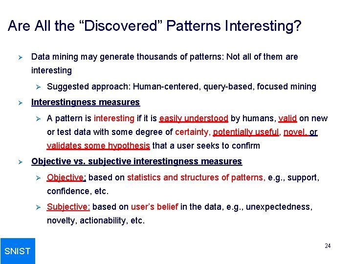
Are All the “Discovered” Patterns Interesting? Ø Data mining may generate thousands of patterns: Not all of them are interesting Ø Ø Suggested approach: Human-centered, query-based, focused mining Interestingness measures Ø A pattern is interesting if it is easily understood by humans, valid on new or test data with some degree of certainty, potentially useful, novel, or validates some hypothesis that a user seeks to confirm Ø Objective vs. subjective interestingness measures Ø Objective: based on statistics and structures of patterns, e. g. , support, confidence, etc. Ø Subjective: based on user’s belief in the data, e. g. , unexpectedness, novelty, actionability, etc. SNIST 24

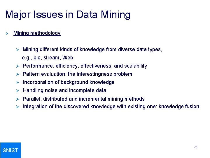
Major Issues in Data Mining Ø Mining methodology Ø Mining different kinds of knowledge from diverse data types, e. g. , bio, stream, Web Ø Performance: efficiency, effectiveness, and scalability Ø Pattern evaluation: the interestingness problem Ø Incorporation of background knowledge Ø Handling noise and incomplete data Ø Parallel, distributed and incremental mining methods Integration of the discovered knowledge with existing one: knowledge fusion Ø SNIST 25

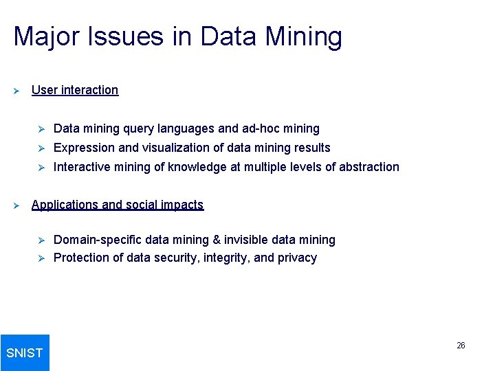
Major Issues in Data Mining Ø Ø User interaction Ø Data mining query languages and ad-hoc mining Ø Expression and visualization of data mining results Ø Interactive mining of knowledge at multiple levels of abstraction Applications and social impacts Ø Ø SNIST Domain-specific data mining & invisible data mining Protection of data security, integrity, and privacy 26

Data Preprocessing Ø Why preprocess the data? Ø Descriptive data summarization Ø Data cleaning Ø Data integration and transformation Ø Data reduction Ø Discretization and concept hierarchy generation SNIST 27

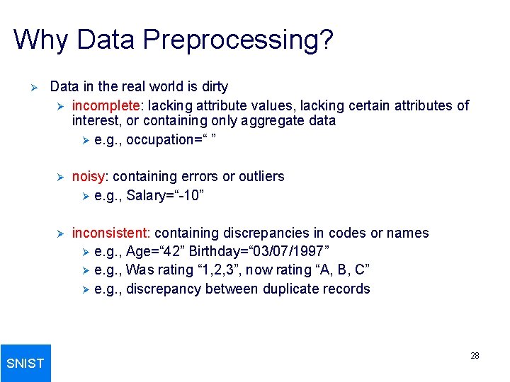
Why Data Preprocessing? Ø SNIST Data in the real world is dirty Ø incomplete: lacking attribute values, lacking certain attributes of interest, or containing only aggregate data Ø e. g. , occupation=“ ” Ø noisy: containing errors or outliers Ø e. g. , Salary=“-10” Ø inconsistent: containing discrepancies in codes or names Ø e. g. , Age=“ 42” Birthday=“ 03/07/1997” Ø e. g. , Was rating “ 1, 2, 3”, now rating “A, B, C” Ø e. g. , discrepancy between duplicate records 28

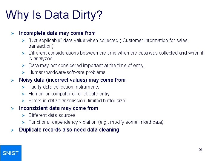
Why Is Data Dirty? Ø Incomplete data may come from Ø Ø Ø Noisy data (incorrect values) may come from Ø Ø Ø SNIST Faulty data collection instruments Human or computer error at data entry Errors in data transmission, limited buffer size Inconsistent data may come from Ø Ø “Not applicable” data value when collected ( Customer information for sales transaction) Different considerations between the time when the data was collected and when it is analyzed. Data may not considered important at the time of entry. Human/hardware/software problems Different data sources Functional dependency violation (e. g. , modify some linked data) Duplicate records also need data cleaning 29

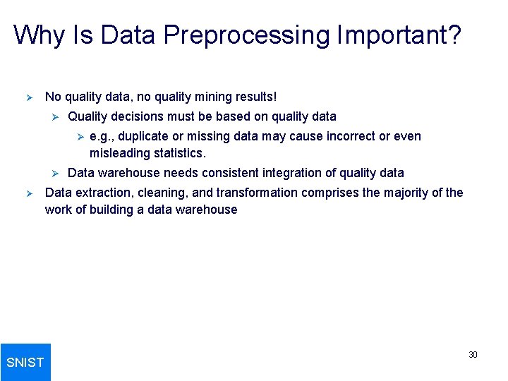
Why Is Data Preprocessing Important? Ø No quality data, no quality mining results! Ø Quality decisions must be based on quality data Ø Ø Ø SNIST e. g. , duplicate or missing data may cause incorrect or even misleading statistics. Data warehouse needs consistent integration of quality data Data extraction, cleaning, and transformation comprises the majority of the work of building a data warehouse 30

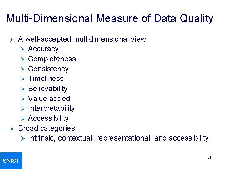
Multi-Dimensional Measure of Data Quality Ø Ø A well-accepted multidimensional view: Ø Accuracy Ø Completeness Ø Consistency Ø Timeliness Ø Believability Ø Value added Ø Interpretability Ø Accessibility Broad categories: Ø Intrinsic, contextual, representational, and accessibility SNIST 31

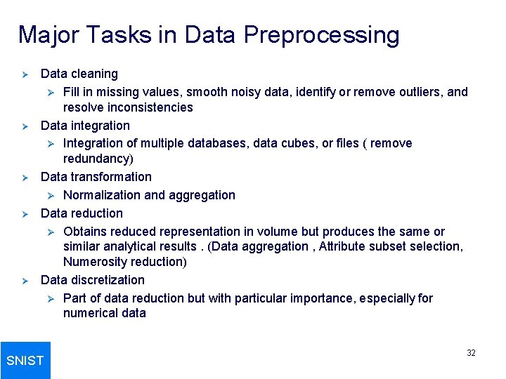
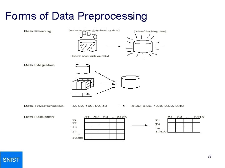
Major Tasks in Data Preprocessing Ø Ø Ø Data cleaning Ø Fill in missing values, smooth noisy data, identify or remove outliers, and resolve inconsistencies Data integration Ø Integration of multiple databases, data cubes, or files ( remove redundancy) Data transformation Ø Normalization and aggregation Data reduction Ø Obtains reduced representation in volume but produces the same or similar analytical results. (Data aggregation , Attribute subset selection, Numerosity reduction) Data discretization Ø Part of data reduction but with particular importance, especially for numerical data SNIST 32

Forms of Data Preprocessing SNIST 33

Data Preprocessing Data cleaning SNIST 34

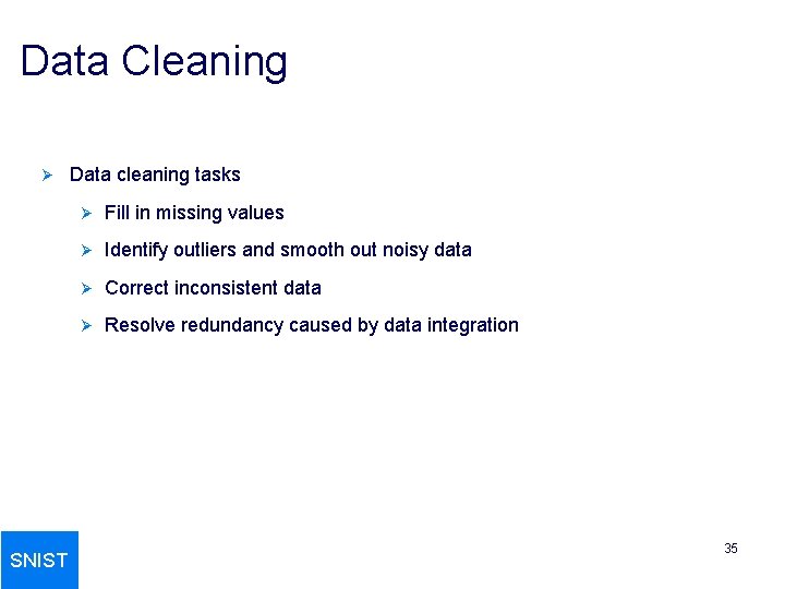
Data Cleaning Ø SNIST Data cleaning tasks Ø Fill in missing values Ø Identify outliers and smooth out noisy data Ø Correct inconsistent data Ø Resolve redundancy caused by data integration 35

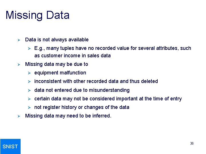
Missing Data Ø Data is not always available Ø Ø Ø SNIST E. g. , many tuples have no recorded value for several attributes, such as customer income in sales data Missing data may be due to Ø equipment malfunction Ø inconsistent with other recorded data and thus deleted Ø data not entered due to misunderstanding Ø certain data may not be considered important at the time of entry Ø not register history or changes of the data Missing data may need to be inferred. 36

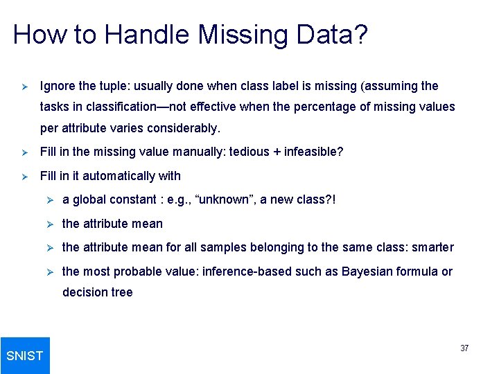
How to Handle Missing Data? Ø Ignore the tuple: usually done when class label is missing (assuming the tasks in classification—not effective when the percentage of missing values per attribute varies considerably. Ø Fill in the missing value manually: tedious + infeasible? Ø Fill in it automatically with Ø a global constant : e. g. , “unknown”, a new class? ! Ø the attribute mean for all samples belonging to the same class: smarter Ø the most probable value: inference-based such as Bayesian formula or decision tree SNIST 37

Noisy Data Ø Ø Ø Noise: random error or variance in a measured variable Incorrect attribute values may due to Ø faulty data collection instruments Ø data entry problems Ø data transmission problems Ø technology limitation Ø inconsistency in naming convention Other data problems which requires data cleaning Ø duplicate records Ø incomplete data Ø inconsistent data SNIST 38

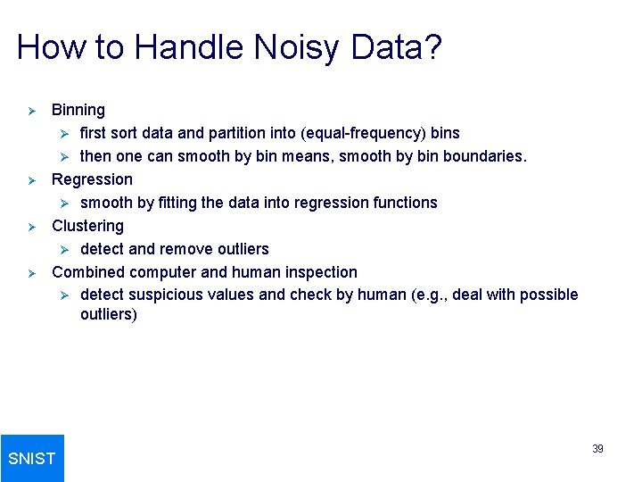
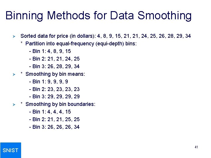
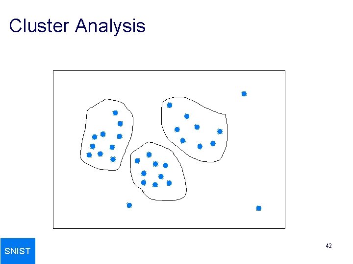
How to Handle Noisy Data? Ø Ø Binning Ø first sort data and partition into (equal-frequency) bins Ø then one can smooth by bin means, smooth by bin boundaries. Regression Ø smooth by fitting the data into regression functions Clustering Ø detect and remove outliers Combined computer and human inspection Ø detect suspicious values and check by human (e. g. , deal with possible outliers) SNIST 39

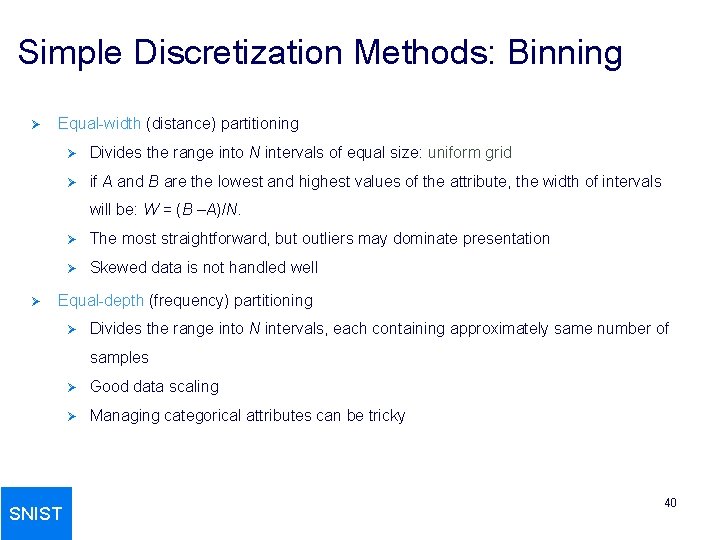
Simple Discretization Methods: Binning Ø Equal-width (distance) partitioning Ø Divides the range into N intervals of equal size: uniform grid Ø if A and B are the lowest and highest values of the attribute, the width of intervals will be: W = (B –A)/N. Ø Ø The most straightforward, but outliers may dominate presentation Ø Skewed data is not handled well Equal-depth (frequency) partitioning Ø Divides the range into N intervals, each containing approximately same number of samples SNIST Ø Good data scaling Ø Managing categorical attributes can be tricky 40

Binning Methods for Data Smoothing Ø Ø Ø SNIST Sorted data for price (in dollars): 4, 8, 9, 15, 21, 24, 25, 26, 28, 29, 34 * Partition into equal-frequency (equi-depth) bins: - Bin 1: 4, 8, 9, 15 - Bin 2: 21, 24, 25 - Bin 3: 26, 28, 29, 34 * Smoothing by bin means: - Bin 1: 9, 9, 9, 9 - Bin 2: 23, 23, 23 - Bin 3: 29, 29, 29 * Smoothing by bin boundaries: - Bin 1: 4, 4, 4, 15 - Bin 2: 21, 25, 25 - Bin 3: 26, 26, 34 41

Cluster Analysis SNIST 42

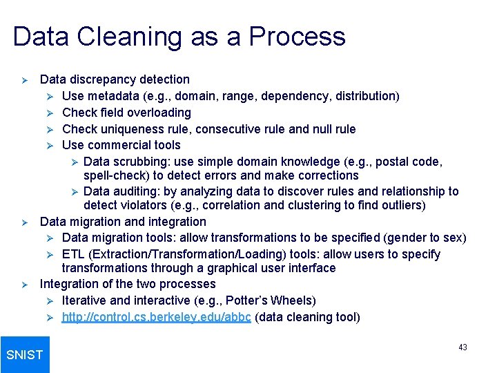
Data Cleaning as a Process Ø Ø Ø Data discrepancy detection Ø Use metadata (e. g. , domain, range, dependency, distribution) Ø Check field overloading Ø Check uniqueness rule, consecutive rule and null rule Ø Use commercial tools Ø Data scrubbing: use simple domain knowledge (e. g. , postal code, spell-check) to detect errors and make corrections Ø Data auditing: by analyzing data to discover rules and relationship to detect violators (e. g. , correlation and clustering to find outliers) Data migration and integration Ø Data migration tools: allow transformations to be specified (gender to sex) Ø ETL (Extraction/Transformation/Loading) tools: allow users to specify transformations through a graphical user interface Integration of the two processes Ø Iterative and interactive (e. g. , Potter’s Wheels) Ø http: //control. cs. berkeley. edu/abbc (data cleaning tool) SNIST 43

Data Preprocessing Data integration and transformation SNIST 44

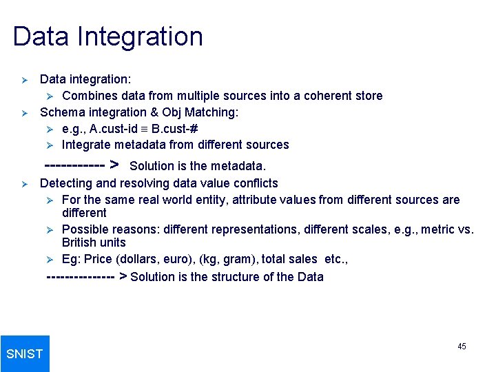
Data Integration Ø Ø Data integration: Ø Combines data from multiple sources into a coherent store Schema integration & Obj Matching: Ø e. g. , A. cust-id B. cust-# Ø Integrate metadata from different sources ------ > Ø Solution is the metadata. Detecting and resolving data value conflicts Ø For the same real world entity, attribute values from different sources are different Ø Possible reasons: different representations, different scales, e. g. , metric vs. British units Ø Eg: Price (dollars, euro), (kg, gram), total sales etc. , -------- > Solution is the structure of the Data SNIST 45

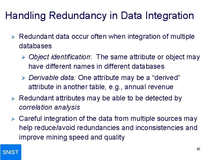
Handling Redundancy in Data Integration Ø Redundant data occur often when integration of multiple databases Ø Object identification: The same attribute or object may have different names in different databases Ø Derivable data: One attribute may be a “derived” attribute in another table, e. g. , annual revenue Ø Redundant attributes may be able to be detected by correlation analysis Ø Careful integration of the data from multiple sources may help reduce/avoid redundancies and inconsistencies and improve mining speed and quality SNIST 46

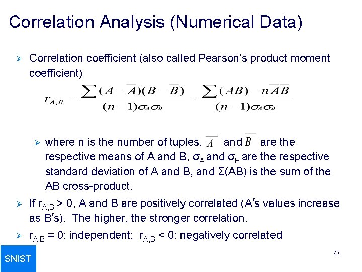
Correlation Analysis (Numerical Data) Ø Correlation coefficient (also called Pearson’s product moment coefficient) Ø where n is the number of tuples, and are the respective means of A and B, σA and σB are the respective standard deviation of A and B, and Σ(AB) is the sum of the AB cross-product. Ø If r. A, B > 0, A and B are positively correlated (A’s values increase as B’s). The higher, the stronger correlation. Ø r. A, B = 0: independent; r. A, B < 0: negatively correlated SNIST 47

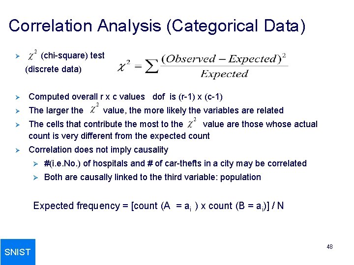
Correlation Analysis (Categorical Data) (chi-square) test Ø (discrete data) Ø Computed overall r x c values dof is (r-1) x (c-1) Ø The larger the Ø The cells that contribute the most to the value are those whose actual count is very different from the expected count Ø Correlation does not imply causality value, the more likely the variables are related Ø #(i. e. No. ) of hospitals and # of car-thefts in a city may be correlated Ø Both are causally linked to the third variable: population Expected frequency = [count (A = ai ) x count (B = ai)] / N SNIST 48

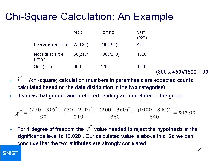
Chi-Square Calculation: An Example Male Female Sum (row) Like science fiction 250(90) 200(360) 450 Not like science fiction 50(210) 1000(840) 1050 Sum(col. ) 300 1200 1500 (300 x 450)/1500 = 90 Ø (chi-square) calculation (numbers in parenthesis are expected counts calculated based on the data distribution in the two categories) Ø It shows that gender and preferred reading are correlated in the group Ø For 1 degree of freedom the value needed to reject the hypothesis at the significance level is 10. 828. Our calculated value is above this. So we can conclude that the two attributes are strongly correlated SNIST 49

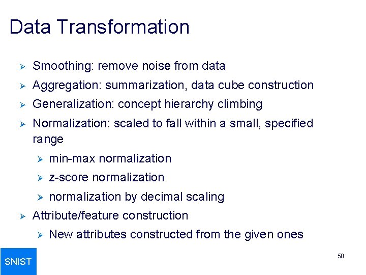
Data Transformation Ø Smoothing: remove noise from data Ø Aggregation: summarization, data cube construction Ø Generalization: concept hierarchy climbing Ø Normalization: scaled to fall within a small, specified range Ø Ø min-max normalization Ø z-score normalization Ø normalization by decimal scaling Attribute/feature construction Ø SNIST New attributes constructed from the given ones 50

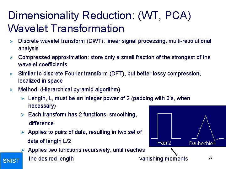
Data Transformation: Normalization Ø Min-max normalization: to [new_min. A, new_max. A] Ø Ø Z-score normalization (μ: mean, σ: standard deviation): Ø Ø Ex. Let income range $12, 000 to $98, 000 normalized to [0. 0, 1. 0]. Then $73, 600 is mapped to Ex. Let μ = 54, 000, σ = 16, 000. Then Normalization by decimal scaling Where j is the smallest integer such that Max(|ν’|) < 1 SNIST 51

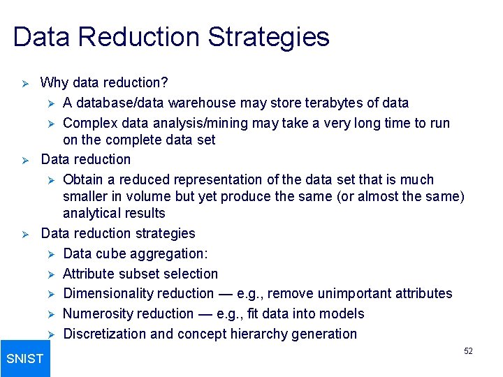
Data Reduction Strategies Ø Ø Ø Why data reduction? Ø A database/data warehouse may store terabytes of data Ø Complex data analysis/mining may take a very long time to run on the complete data set Data reduction Ø Obtain a reduced representation of the data set that is much smaller in volume but yet produce the same (or almost the same) analytical results Data reduction strategies Ø Data cube aggregation: Ø Attribute subset selection Ø Dimensionality reduction — e. g. , remove unimportant attributes Ø Numerosity reduction — e. g. , fit data into models Ø Discretization and concept hierarchy generation SNIST 52

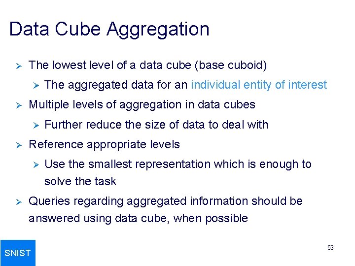
Data Cube Aggregation Ø The lowest level of a data cube (base cuboid) Ø Ø Multiple levels of aggregation in data cubes Ø Ø Further reduce the size of data to deal with Reference appropriate levels Ø Ø The aggregated data for an individual entity of interest Use the smallest representation which is enough to solve the task Queries regarding aggregated information should be answered using data cube, when possible SNIST 53

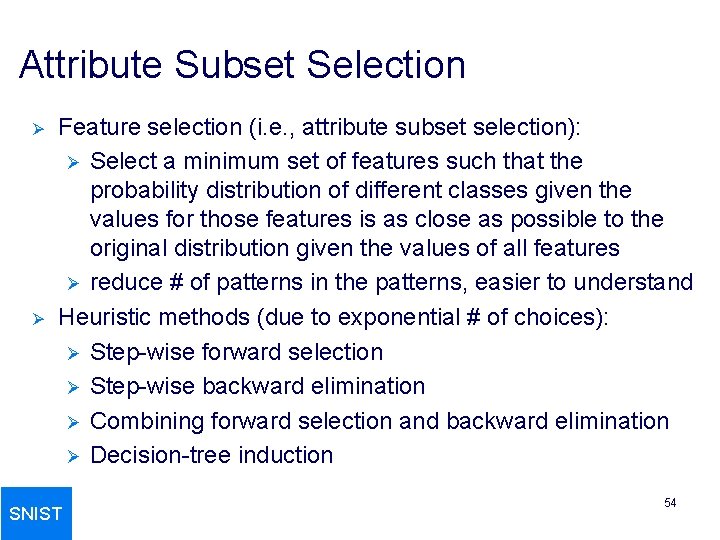
Attribute Subset Selection Ø Ø Feature selection (i. e. , attribute subset selection): Ø Select a minimum set of features such that the probability distribution of different classes given the values for those features is as close as possible to the original distribution given the values of all features Ø reduce # of patterns in the patterns, easier to understand Heuristic methods (due to exponential # of choices): Ø Step-wise forward selection Ø Step-wise backward elimination Ø Combining forward selection and backward elimination Ø Decision-tree induction SNIST 54

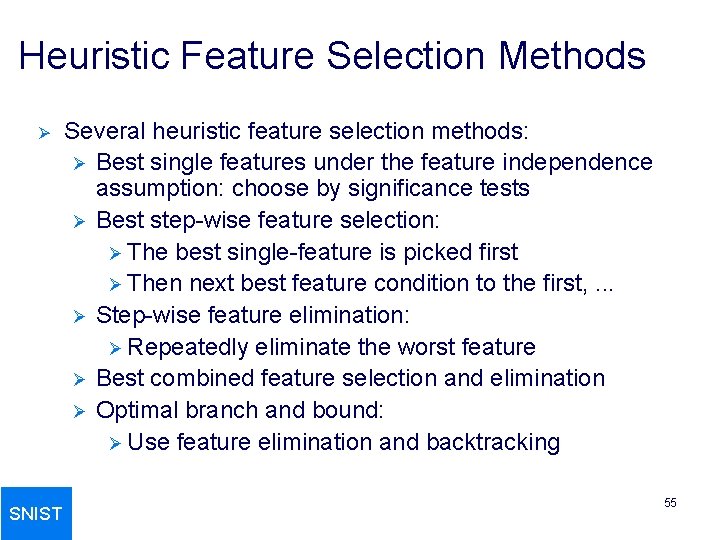
Heuristic Feature Selection Methods Ø SNIST Several heuristic feature selection methods: Ø Best single features under the feature independence assumption: choose by significance tests Ø Best step-wise feature selection: Ø The best single-feature is picked first Ø Then next best feature condition to the first, . . . Ø Step-wise feature elimination: Ø Repeatedly eliminate the worst feature Ø Best combined feature selection and elimination Ø Optimal branch and bound: Ø Use feature elimination and backtracking 55

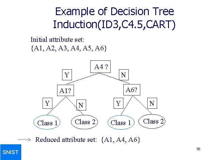
Example of Decision Tree Induction(ID 3, C 4. 5, CART) Initial attribute set: {A 1, A 2, A 3, A 4, A 5, A 6} A 4 ? Y N A 6? A 1? Y Class 1 > SNIST N Class 2 Y Class 1 N Class 2 Reduced attribute set: {A 1, A 4, A 6} 56

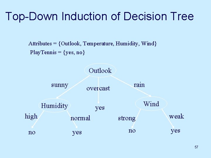
Top-Down Induction of Decision Tree Attributes = {Outlook, Temperature, Humidity, Wind} Play. Tennis = {yes, no} Outlook sunny overcast Humidity high no rain Wind yes normal yes strong no weak yes 57

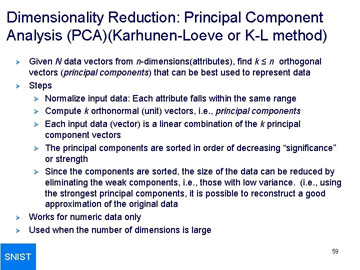
Dimensionality Reduction: (WT, PCA) Wavelet Transformation Ø Discrete wavelet transform (DWT): linear signal processing, multi-resolutional analysis Ø Compressed approximation: store only a small fraction of the strongest of the wavelet coefficients Ø Similar to discrete Fourier transform (DFT), but better lossy compression, localized in space Ø Method: (Hierarchical pyramid algorithm) Ø Length, L, must be an integer power of 2 (padding with 0’s, when necessary) Ø Each transform has 2 functions: smoothing, difference Ø Applies to pairs of data, resulting in two set of data of length L/2 Ø SNIST Haar 2 Daubechie 4 Applies two functions recursively, until reaches the desired length vanishing moments 58

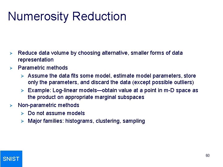
Dimensionality Reduction: Principal Component Analysis (PCA)(Karhunen-Loeve or K-L method) Ø Ø Given N data vectors from n-dimensions(attributes), find k ≤ n orthogonal vectors (principal components) that can be best used to represent data Steps Ø Normalize input data: Each attribute falls within the same range Ø Compute k orthonormal (unit) vectors, i. e. , principal components Ø Each input data (vector) is a linear combination of the k principal component vectors Ø The principal components are sorted in order of decreasing “significance” or strength Ø Since the components are sorted, the size of the data can be reduced by eliminating the weak components, i. e. , those with low variance. (i. e. , using the strongest principal components, it is possible to reconstruct a good approximation of the original data Works for numeric data only Used when the number of dimensions is large SNIST 59

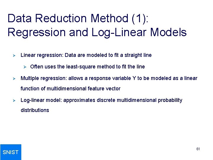
Numerosity Reduction Ø Ø Ø Reduce data volume by choosing alternative, smaller forms of data representation Parametric methods Ø Assume the data fits some model, estimate model parameters, store only the parameters, and discard the data (except possible outliers) Ø Example: Log-linear models—obtain value at a point in m-D space as the product on appropriate marginal subspaces Non-parametric methods Ø Do not assume models Ø Major families: histograms, clustering, sampling SNIST 60

Data Reduction Method (1): Regression and Log-Linear Models Ø Linear regression: Data are modeled to fit a straight line Ø Ø Often uses the least-square method to fit the line Multiple regression: allows a response variable Y to be modeled as a linear function of multidimensional feature vector Ø Log-linear model: approximates discrete multidimensional probability distributions SNIST 61

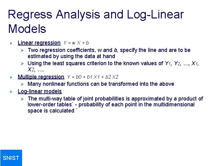
Regress Analysis and Log-Linear Models Ø Ø Ø Linear regression: Y = w X + b Ø Two regression coefficients, w and b, specify the line and are to be estimated by using the data at hand Ø Using the least squares criterion to the known values of Y 1, Y 2, …, X 1, X 2, …. Multiple regression: Y = b 0 + b 1 X 1 + b 2 X 2. Ø Many nonlinear functions can be transformed into the above Log-linear models: Ø The multi-way table of joint probabilities is approximated by a product of lower-order tables` - probability of each point in the multidimensional space is calculated ` SNIST

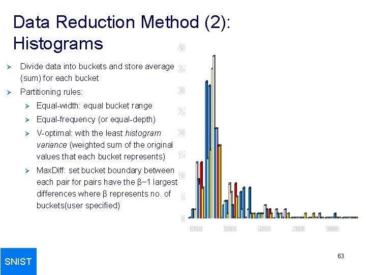
Data Reduction Method (2): Histograms Ø Divide data into buckets and store average (sum) for each bucket Ø Partitioning rules: Ø Equal-width: equal bucket range Ø Equal-frequency (or equal-depth) Ø V-optimal: with the least histogram variance (weighted sum of the original values that each bucket represents) Ø Max. Diff: set bucket boundary between each pair for pairs have the β– 1 largest differences where β represents no. of buckets(user specified) SNIST 63

Data Reduction Method (3): Clustering Ø Partition data set into clusters based on similarity, and store cluster representation (e. g. , centroid and diameter) only Ø Can be very effective if data is clustered but not if data is “smeared” Ø Can have hierarchical clustering and be stored in multi-dimensional index tree structures Ø There are many choices of clustering definitions and clustering algorithms Ø Objects with in a cluster are similar Ø Similarity is based on distance function SNIST 64

Data Reduction Method (4): Sampling Ø Ø Sampling: obtaining a small sample s to represent the whole data set N Allow a mining algorithm to run in complexity that is potentially sub-linear to the size of the data Choose a representative subset of the data Ø Simple random sampling may have very poor performance in the presence of skew Develop adaptive sampling methods Ø Stratified sampling: Approximate the percentage of each class (or subpopulation of interest) in the overall database Ø Used in conjunction with skewed data Ø Ø SNIST Note: Sampling may not reduce database I/Os (page at a time) 65

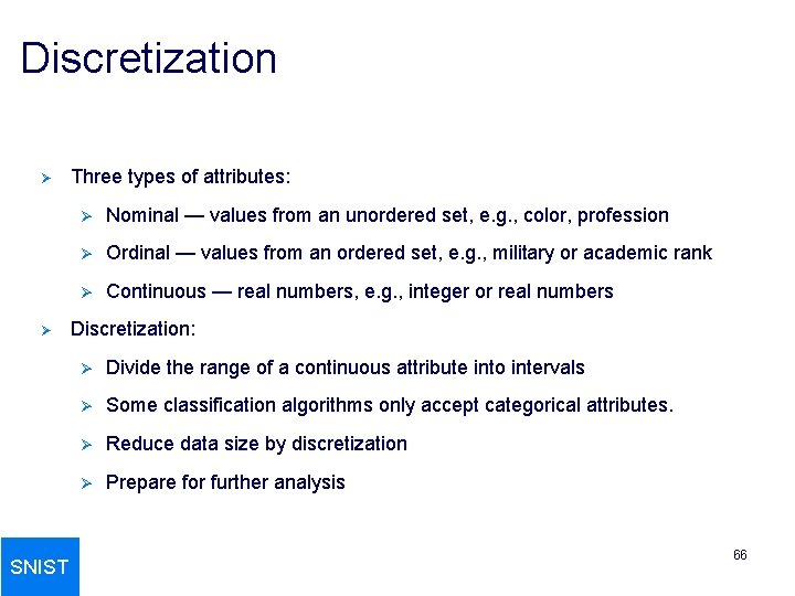
Discretization Ø Ø SNIST Three types of attributes: Ø Nominal — values from an unordered set, e. g. , color, profession Ø Ordinal — values from an ordered set, e. g. , military or academic rank Ø Continuous — real numbers, e. g. , integer or real numbers Discretization: Ø Divide the range of a continuous attribute into intervals Ø Some classification algorithms only accept categorical attributes. Ø Reduce data size by discretization Ø Prepare for further analysis 66

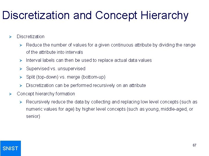
Discretization and Concept Hierarchy Ø Discretization Ø Reduce the number of values for a given continuous attribute by dividing the range of the attribute into intervals Ø Ø Interval labels can then be used to replace actual data values Ø Supervised vs. unsupervised Ø Split (top-down) vs. merge (bottom-up) Ø Discretization can be performed recursively on an attribute Concept hierarchy formation Ø Recursively reduce the data by collecting and replacing low level concepts (such as numeric values for age) by higher level concepts (such as young, middle-aged, or senior) SNIST 67

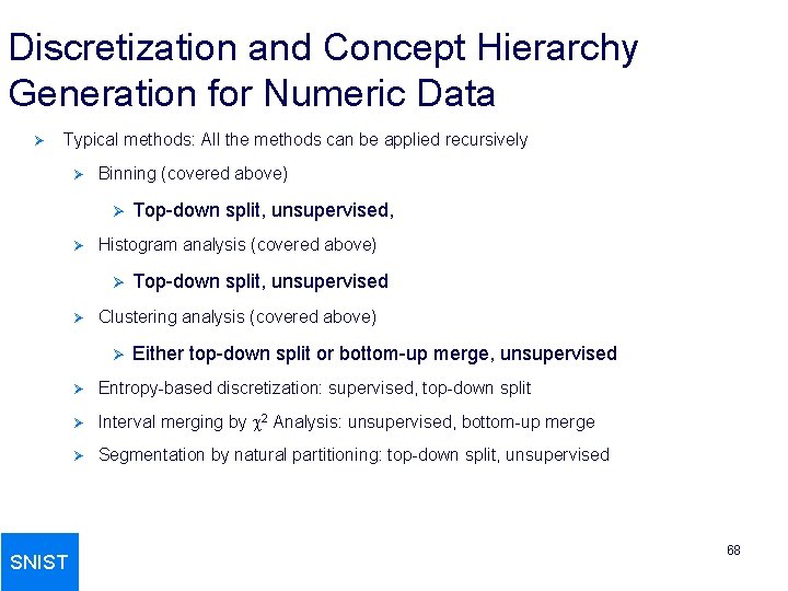
Discretization and Concept Hierarchy Generation for Numeric Data Ø Typical methods: All the methods can be applied recursively Ø Binning (covered above) Ø Ø Histogram analysis (covered above) Ø Ø Top-down split, unsupervised Clustering analysis (covered above) Ø SNIST Top-down split, unsupervised, Either top-down split or bottom-up merge, unsupervised Ø Entropy-based discretization: supervised, top-down split Ø Interval merging by 2 Analysis: unsupervised, bottom-up merge Ø Segmentation by natural partitioning: top-down split, unsupervised 68

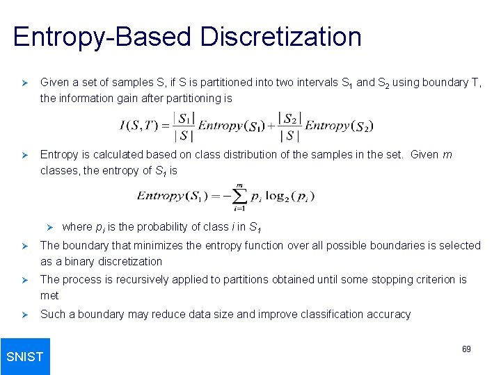
Entropy-Based Discretization Ø Given a set of samples S, if S is partitioned into two intervals S 1 and S 2 using boundary T, the information gain after partitioning is Ø Entropy is calculated based on class distribution of the samples in the set. Given m classes, the entropy of S 1 is Ø where pi is the probability of class i in S 1 Ø The boundary that minimizes the entropy function over all possible boundaries is selected as a binary discretization Ø The process is recursively applied to partitions obtained until some stopping criterion is met Ø Such a boundary may reduce data size and improve classification accuracy SNIST 69

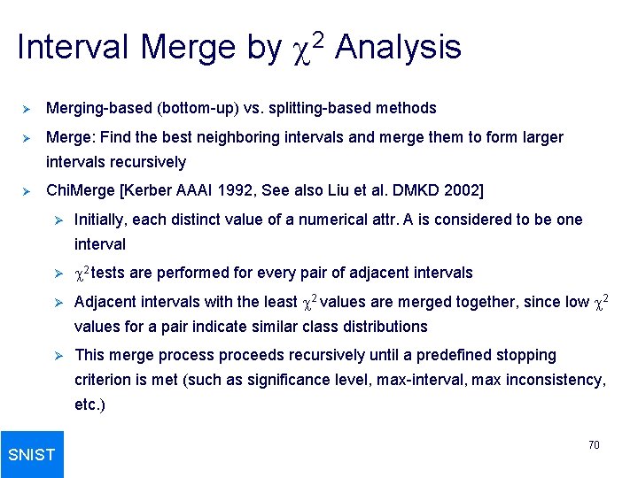
Interval Merge by 2 Analysis Ø Merging-based (bottom-up) vs. splitting-based methods Ø Merge: Find the best neighboring intervals and merge them to form larger intervals recursively Ø Chi. Merge [Kerber AAAI 1992, See also Liu et al. DMKD 2002] Ø Initially, each distinct value of a numerical attr. A is considered to be one interval Ø 2 tests are performed for every pair of adjacent intervals Ø Adjacent intervals with the least 2 values are merged together, since low 2 values for a pair indicate similar class distributions Ø This merge process proceeds recursively until a predefined stopping criterion is met (such as significance level, max-interval, max inconsistency, etc. ) SNIST 70

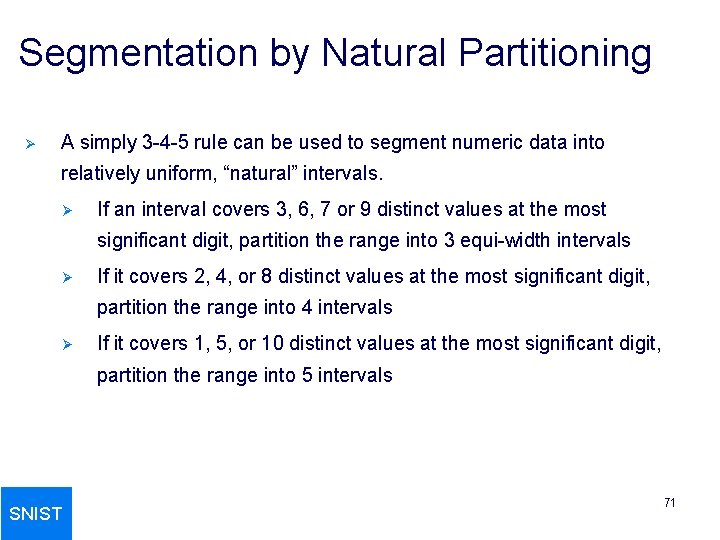
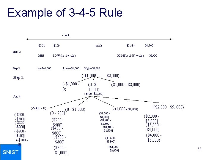
Segmentation by Natural Partitioning Ø A simply 3 -4 -5 rule can be used to segment numeric data into relatively uniform, “natural” intervals. Ø If an interval covers 3, 6, 7 or 9 distinct values at the most significant digit, partition the range into 3 equi-width intervals Ø If it covers 2, 4, or 8 distinct values at the most significant digit, partition the range into 4 intervals Ø If it covers 1, 5, or 10 distinct values at the most significant digit, partition the range into 5 intervals SNIST 71

Example of 3 -4 -5 Rule count -$351 -$159 profit MIN LOW (i. e, 5%-tile) $1, 838 $4, 700 Step 1: Step 2: msd=1, 000 Low=-$1, 000 HIGH(i. e, 95%-0 tile) High=$2, 000 (-$1, 000…. . - $2, 000) Step 3: (-$1, 000 0) (-$400 - 0) SNIST (0 -$ 1, 000) ($1, 000 - $2, 000) (-$400 -$5, 000) Step 4: (-$400 -$300] (-$300 -$200] (-$200 -$100] (-$100 0] MAX (0 - 200] (0 - $1, 000) ($200 $400] ($400 $600] ($600 $800] ($800 $1, 000] ($1, 000 - $2, 000) ($1, 000 $1, 200] ($1, 200 $1, 400) ($1, 400 $1, 600] ($1, 600 $1, 800] ($1, 800 $2, 000] ($2, 000 - $5, 000) ($2, 000 $3, 000] ($3, 000 $4, 000] ($4, 000 $5, 000) 72

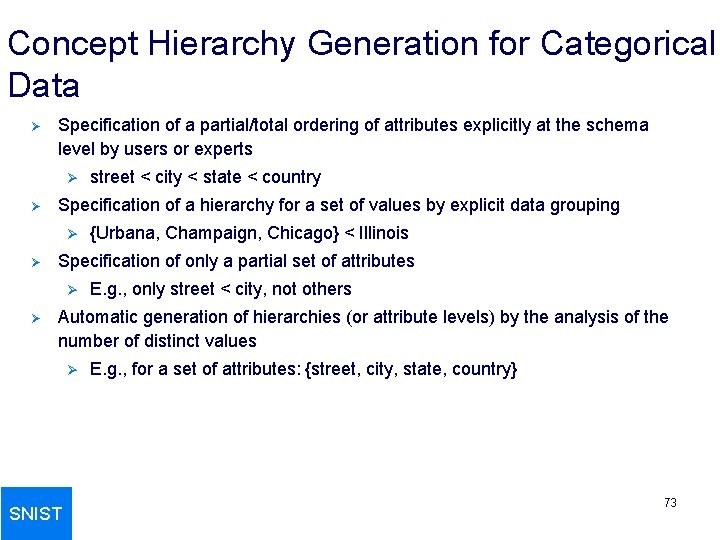
Concept Hierarchy Generation for Categorical Data Ø Specification of a partial/total ordering of attributes explicitly at the schema level by users or experts Ø Ø Specification of a hierarchy for a set of values by explicit data grouping Ø Ø {Urbana, Champaign, Chicago} < Illinois Specification of only a partial set of attributes Ø Ø street < city < state < country E. g. , only street < city, not others Automatic generation of hierarchies (or attribute levels) by the analysis of the number of distinct values Ø SNIST E. g. , for a set of attributes: {street, city, state, country} 73

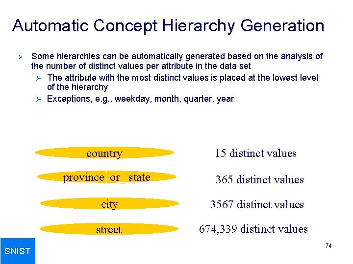
Automatic Concept Hierarchy Generation Ø Some hierarchies can be automatically generated based on the analysis of the number of distinct values per attribute in the data set Ø The attribute with the most distinct values is placed at the lowest level of the hierarchy Ø Exceptions, e. g. , weekday, month, quarter, year country province_or_ state 365 distinct values city 3567 distinct values street SNIST 15 distinct values 674, 339 distinct values 74