Data Mining Concepts and Techniques Chapter 3 Data

Data Mining: Concepts and Techniques — Chapter 3 — Data Preprocessing 1

Chapter 3: Data Preprocessing n Data Preprocessing: An Overview n Data Quality n Major Tasks in Data Preprocessing n Data Cleaning n Data Integration n Data Reduction n Data Transformation and Data Discretization n Summary 2

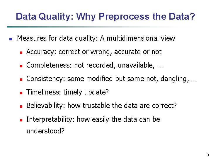
Data Quality: Why Preprocess the Data? n Measures for data quality: A multidimensional view n Accuracy: correct or wrong, accurate or not n Completeness: not recorded, unavailable, … n Consistency: some modified but some not, dangling, … n Timeliness: timely update? n Believability: how trustable the data are correct? n Interpretability: how easily the data can be understood? 3

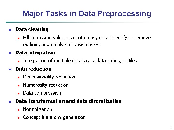
Major Tasks in Data Preprocessing n Data cleaning n n Data integration n Fill in missing values, smooth noisy data, identify or remove outliers, and resolve inconsistencies Integration of multiple databases, data cubes, or files Data reduction n Dimensionality reduction n Numerosity reduction n Data compression Data transformation and data discretization n Normalization n Concept hierarchy generation 4

Chapter 3: Data Preprocessing n Data Preprocessing: An Overview n Data Quality n Major Tasks in Data Preprocessing n Data Cleaning n Data Integration n Data Reduction n Data Transformation and Data Discretization n Summary 5

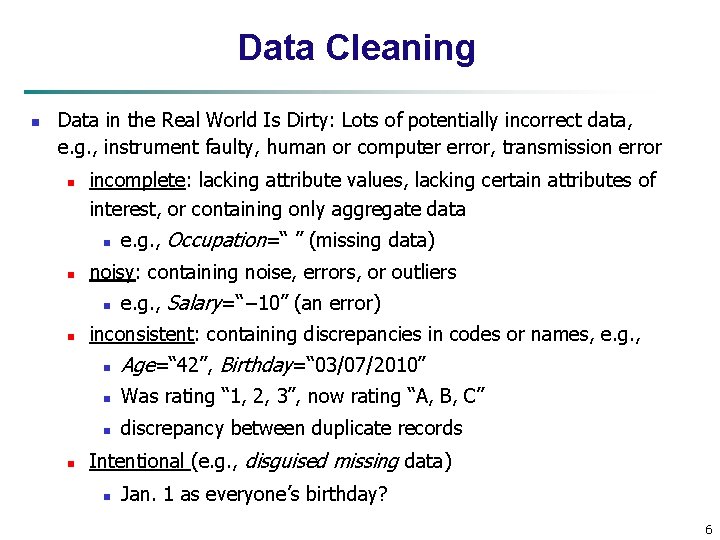
Data Cleaning n Data in the Real World Is Dirty: Lots of potentially incorrect data, e. g. , instrument faulty, human or computer error, transmission error n incomplete: lacking attribute values, lacking certain attributes of interest, or containing only aggregate data n n noisy: containing noise, errors, or outliers n n n e. g. , Occupation=“ ” (missing data) e. g. , Salary=“− 10” (an error) inconsistent: containing discrepancies in codes or names, e. g. , n Age=“ 42”, Birthday=“ 03/07/2010” n Was rating “ 1, 2, 3”, now rating “A, B, C” n discrepancy between duplicate records Intentional (e. g. , disguised missing data) n Jan. 1 as everyone’s birthday? 6

Incomplete (Missing) Data n Data is not always available n n Missing data may be due to n equipment malfunction n inconsistent with other recorded data and thus deleted n data not entered due to misunderstanding n n n E. g. , many tuples have no recorded value for several attributes, such as customer income in sales data certain data may not be considered important at the time of entry not register history or changes of the data Missing data may need to be inferred 7

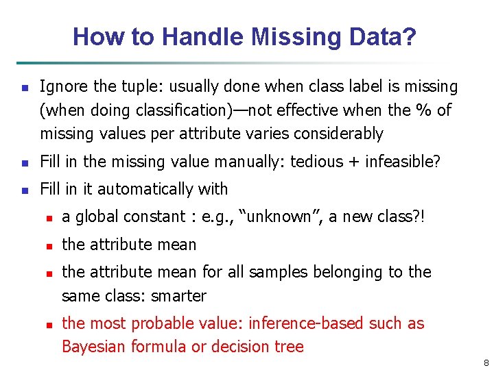
How to Handle Missing Data? n Ignore the tuple: usually done when class label is missing (when doing classification)—not effective when the % of missing values per attribute varies considerably n Fill in the missing value manually: tedious + infeasible? n Fill in it automatically with n a global constant : e. g. , “unknown”, a new class? ! n the attribute mean n n the attribute mean for all samples belonging to the same class: smarter the most probable value: inference-based such as Bayesian formula or decision tree 8

Noisy Data n n n Noise: random error or variance in a measured variable Incorrect attribute values may be due to n faulty data collection instruments n data entry problems n data transmission problems n technology limitation n inconsistency in naming convention Other data problems which require data cleaning n duplicate records n incomplete data n inconsistent data 9

How to Handle Noisy Data? n n Binning n first sort data and partition into (equal-frequency) bins n then one can smooth by bin means, smooth by bin median, smooth by bin boundaries, etc. Regression n smooth by fitting the data into regression functions Clustering n detect and remove outliers Combined computer and human inspection n detect suspicious values and check by human (e. g. , deal with possible outliers) 10

Data Cleaning as a Process n n n Data discrepancy detection n Use metadata (e. g. , domain, range, dependency, distribution) n Check field overloading (Field overloading is another source of errors that typically results when developers squeeze new attribute) n Check uniqueness rule, consecutive rule and null rule n Use commercial tools n Data scrubbing: use simple domain knowledge (e. g. , postal code, spell-check) to detect errors and make corrections n Data auditing: by analyzing data to discover rules and relationship to detect violators (e. g. , correlation and clustering to find outliers) Data migration and integration n Data migration tools: allow transformations to be specified n ETL (Extraction/Transformation/Loading) tools: allow users to specify transformations through a graphical user interface Integration of the two processes n Iterative and interactive 11

Chapter 3: Data Preprocessing n Data Preprocessing: An Overview n Data Quality n Major Tasks in Data Preprocessing n Data Cleaning n Data Integration n Data Reduction n Data Transformation and Data Discretization n Summary 12

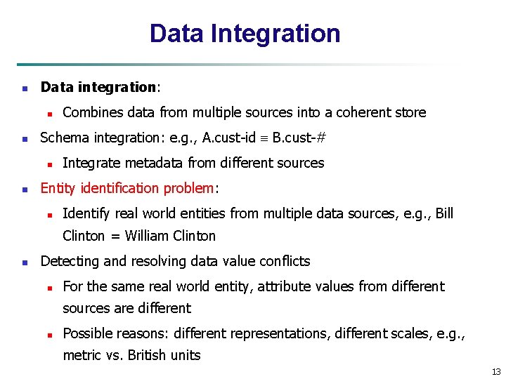
Data Integration n Data integration: n n Schema integration: e. g. , A. cust-id B. cust-# n n Combines data from multiple sources into a coherent store Integrate metadata from different sources Entity identification problem: n Identify real world entities from multiple data sources, e. g. , Bill Clinton = William Clinton n Detecting and resolving data value conflicts n For the same real world entity, attribute values from different sources are different n Possible reasons: different representations, different scales, e. g. , metric vs. British units 13

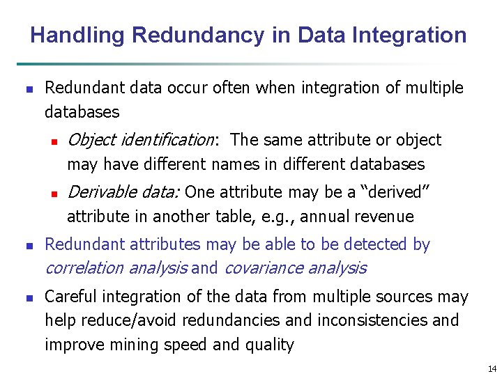
Handling Redundancy in Data Integration n Redundant data occur often when integration of multiple databases n Object identification: The same attribute or object may have different names in different databases n Derivable data: One attribute may be a “derived” attribute in another table, e. g. , annual revenue n n Redundant attributes may be able to be detected by correlation analysis and covariance analysis Careful integration of the data from multiple sources may help reduce/avoid redundancies and inconsistencies and improve mining speed and quality 14

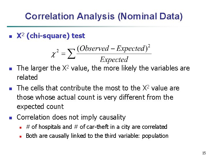
Correlation Analysis (Nominal Data) n n Χ 2 (chi-square) test The larger the Χ 2 value, the more likely the variables are related The cells that contribute the most to the Χ 2 value are those whose actual count is very different from the expected count Correlation does not imply causality n # of hospitals and # of car-theft in a city are correlated n Both are causally linked to the third variable: population 15

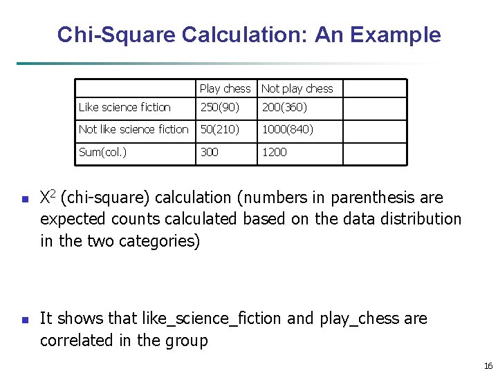
Chi-Square Calculation: An Example n n Play chess Not play chess Like science fiction 250(90) 200(360) Not like science fiction 50(210) 1000(840) Sum(col. ) 300 1200 Χ 2 (chi-square) calculation (numbers in parenthesis are expected counts calculated based on the data distribution in the two categories) It shows that like_science_fiction and play_chess are correlated in the group 16

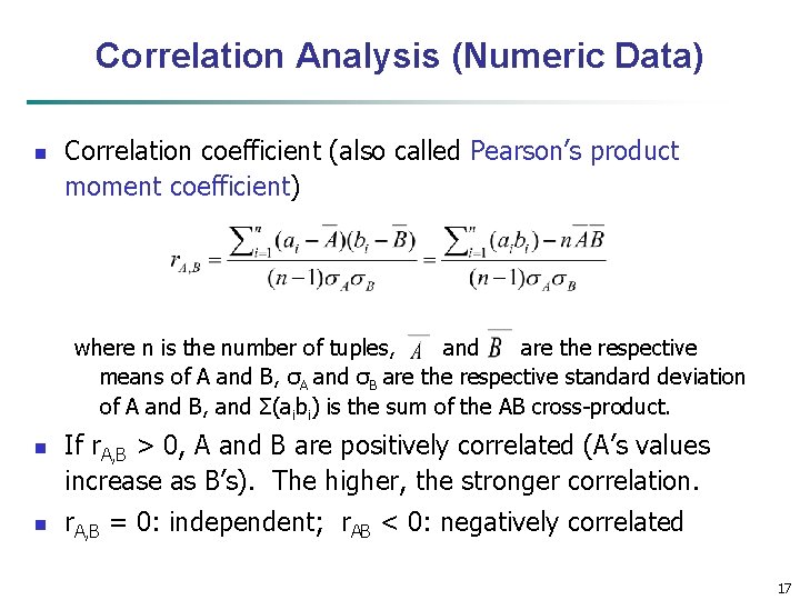
Correlation Analysis (Numeric Data) n Correlation coefficient (also called Pearson’s product moment coefficient) where n is the number of tuples, and are the respective means of A and B, σA and σB are the respective standard deviation of A and B, and Σ(aibi) is the sum of the AB cross-product. n n If r. A, B > 0, A and B are positively correlated (A’s values increase as B’s). The higher, the stronger correlation. r. A, B = 0: independent; r. AB < 0: negatively correlated 17

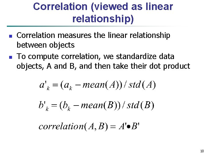
Correlation (viewed as linear relationship) n n Correlation measures the linear relationship between objects To compute correlation, we standardize data objects, A and B, and then take their dot product 18

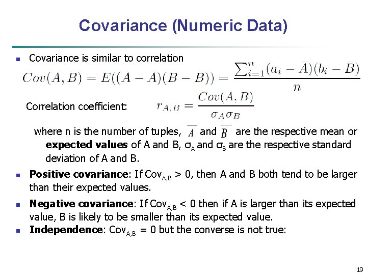
Covariance (Numeric Data) n Covariance is similar to correlation Correlation coefficient: where n is the number of tuples, and are the respective mean or expected values of A and B, σA and σB are the respective standard deviation of A and B. n n n Positive covariance: If Cov. A, B > 0, then A and B both tend to be larger than their expected values. Negative covariance: If Cov. A, B < 0 then if A is larger than its expected value, B is likely to be smaller than its expected value. Independence: Cov. A, B = 0 but the converse is not true: 19

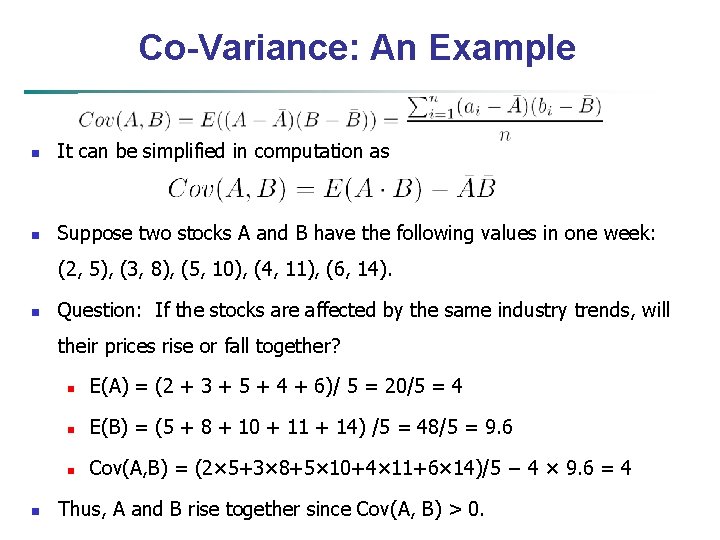
Co-Variance: An Example n It can be simplified in computation as n Suppose two stocks A and B have the following values in one week: (2, 5), (3, 8), (5, 10), (4, 11), (6, 14). n Question: If the stocks are affected by the same industry trends, will their prices rise or fall together? n n E(A) = (2 + 3 + 5 + 4 + 6)/ 5 = 20/5 = 4 n E(B) = (5 + 8 + 10 + 11 + 14) /5 = 48/5 = 9. 6 n Cov(A, B) = (2× 5+3× 8+5× 10+4× 11+6× 14)/5 − 4 × 9. 6 = 4 Thus, A and B rise together since Cov(A, B) > 0.

Chapter 3: Data Preprocessing n Data Preprocessing: An Overview n Data Quality n Major Tasks in Data Preprocessing n Data Cleaning n Data Integration n Data Reduction n Data Transformation and Data Discretization n Summary 21

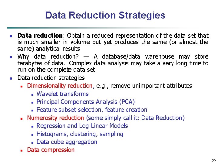
Data Reduction Strategies n n n Data reduction: Obtain a reduced representation of the data set that is much smaller in volume but yet produces the same (or almost the same) analytical results Why data reduction? — A database/data warehouse may store terabytes of data. Complex data analysis may take a very long time to run on the complete data set. Data reduction strategies n Dimensionality reduction, e. g. , remove unimportant attributes n Wavelet transforms n Principal Components Analysis (PCA) n Feature subset selection, feature creation n Numerosity reduction (some simply call it: Data Reduction) n Regression and Log-Linear Models n Histograms, clustering, sampling n Data cube aggregation n Data compression 22

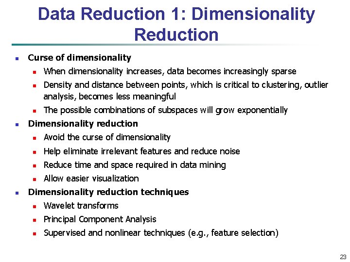
Data Reduction 1: Dimensionality Reduction n Curse of dimensionality n n n When dimensionality increases, data becomes increasingly sparse Density and distance between points, which is critical to clustering, outlier analysis, becomes less meaningful The possible combinations of subspaces will grow exponentially Dimensionality reduction n Avoid the curse of dimensionality n Help eliminate irrelevant features and reduce noise n Reduce time and space required in data mining n Allow easier visualization Dimensionality reduction techniques n Wavelet transforms n Principal Component Analysis n Supervised and nonlinear techniques (e. g. , feature selection) 23

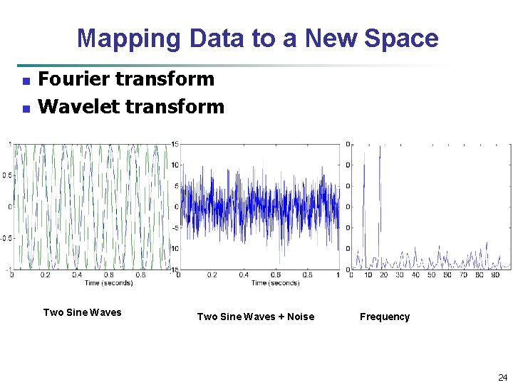
Mapping Data to a New Space n n Fourier transform Wavelet transform Two Sine Waves + Noise Frequency 24

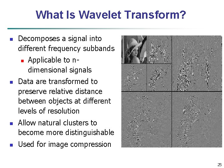
What Is Wavelet Transform? n Decomposes a signal into different frequency subbands n n Applicable to ndimensional signals Data are transformed to preserve relative distance between objects at different levels of resolution Allow natural clusters to become more distinguishable Used for image compression 25

Why Wavelet Transform? n n n Use hat-shape filters n Emphasize region where points cluster n Suppress weaker information in their boundaries Effective removal of outliers n Insensitive to noise, insensitive to input order Multi-resolution n Detect arbitrary shaped clusters at different scales Efficient n Complexity O(N) Only applicable to low dimensional data 26

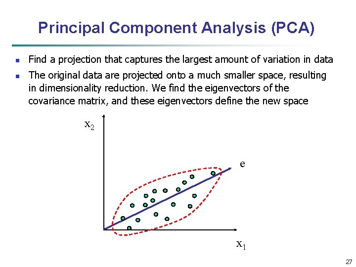
Principal Component Analysis (PCA) n n Find a projection that captures the largest amount of variation in data The original data are projected onto a much smaller space, resulting in dimensionality reduction. We find the eigenvectors of the covariance matrix, and these eigenvectors define the new space x 2 e x 1 27

Attribute Subset Selection n Another way to reduce dimensionality of data: n Redundant attributes n Irrelevant attributes 28

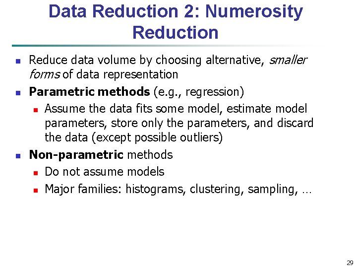
Data Reduction 2: Numerosity Reduction n Reduce data volume by choosing alternative, smaller forms of data representation Parametric methods (e. g. , regression) n Assume the data fits some model, estimate model parameters, store only the parameters, and discard the data (except possible outliers) Non-parametric methods n Do not assume models n Major families: histograms, clustering, sampling, … 29

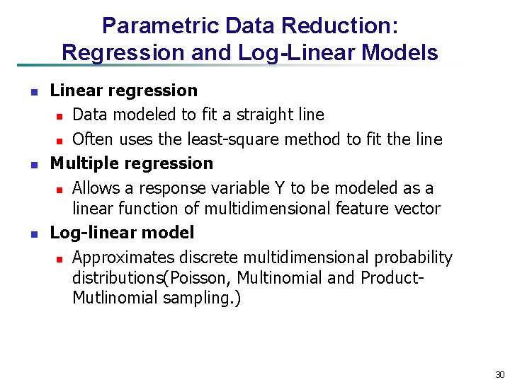
Parametric Data Reduction: Regression and Log-Linear Models n n n Linear regression n Data modeled to fit a straight line n Often uses the least-square method to fit the line Multiple regression n Allows a response variable Y to be modeled as a linear function of multidimensional feature vector Log-linear model n Approximates discrete multidimensional probability distributions(Poisson, Multinomial and Product. Mutlinomial sampling. ) 30

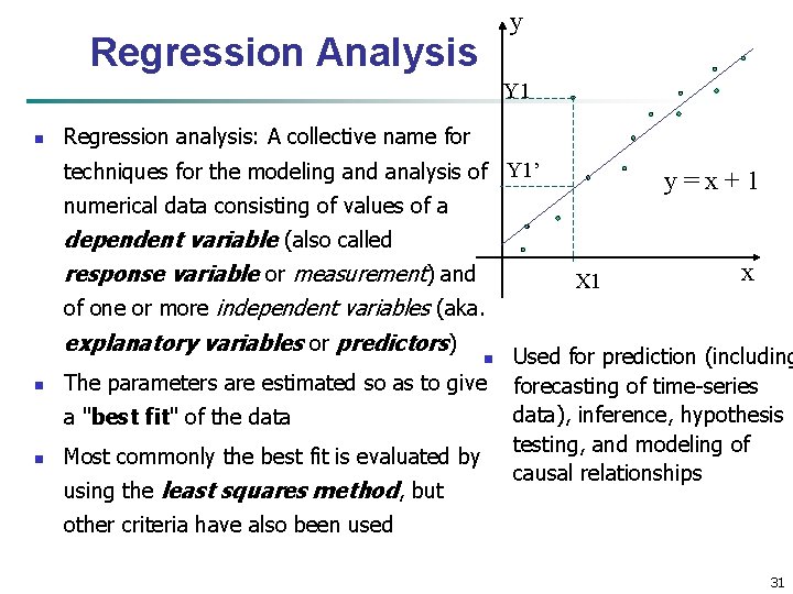
y Regression Analysis Y 1 n Regression analysis: A collective name for techniques for the modeling and analysis of Y 1’ y=x+1 numerical data consisting of values of a dependent variable (also called response variable or measurement) and of one or more independent variables (aka. explanatory variables or predictors) n n The parameters are estimated so as to give a "best fit" of the data n Most commonly the best fit is evaluated by using the least squares method, but X 1 x Used for prediction (including forecasting of time-series data), inference, hypothesis testing, and modeling of causal relationships other criteria have also been used 31

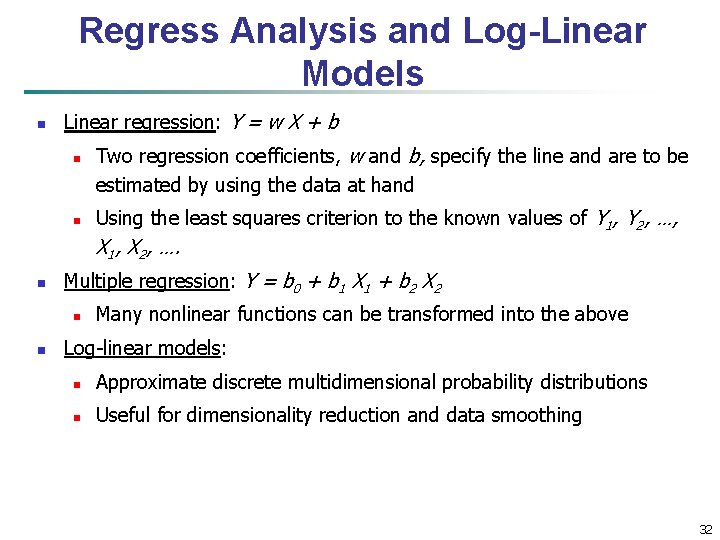
Regress Analysis and Log-Linear Models n Linear regression: Y = w X + b n n Two regression coefficients, w and b, specify the line and are to be estimated by using the data at hand Using the least squares criterion to the known values of Y 1, Y 2, …, X 1, X 2, …. n Multiple regression: Y = b 0 + b 1 X 1 + b 2 X 2 n n Many nonlinear functions can be transformed into the above Log-linear models: n Approximate discrete multidimensional probability distributions n Useful for dimensionality reduction and data smoothing 32

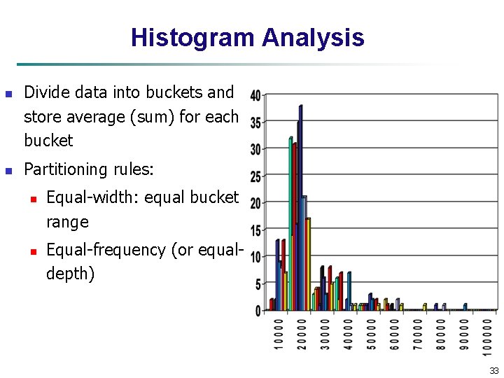
Histogram Analysis n n Divide data into buckets and store average (sum) for each bucket Partitioning rules: n n Equal-width: equal bucket range Equal-frequency (or equaldepth) 33

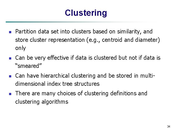
Clustering n n Partition data set into clusters based on similarity, and store cluster representation (e. g. , centroid and diameter) only Can be very effective if data is clustered but not if data is “smeared” Can have hierarchical clustering and be stored in multidimensional index tree structures There are many choices of clustering definitions and clustering algorithms 34

Sampling n n n Sampling: obtaining a small sample s to represent the whole data set N Allow a mining algorithm to run in complexity that is potentially sub-linear to the size of the data Key principle: Choose a representative subset of the data n n n Simple random sampling may have very poor performance in the presence of skew Develop adaptive sampling methods, e. g. , stratified sampling: Note: Sampling may not reduce database I/Os (page at a time) 35

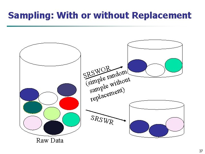
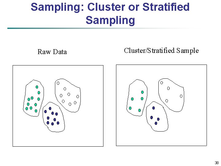
Types of Sampling n n Simple random sampling n There is an equal probability of selecting any particular item Sampling without replacement n Once an object is selected, it is removed from the population Sampling with replacement n A selected object is not removed from the population Stratified sampling: n Partition the data set, and draw samples from each partition (proportionally, i. e. , approximately the same percentage of the data) 36

Sampling: With or without Replacement R O W SRS le random t p u o m i h t s ( wi e l p sam ment) e c a l p re SRSW R Raw Data 37

Sampling: Cluster or Stratified Sampling Raw Data Cluster/Stratified Sample 38

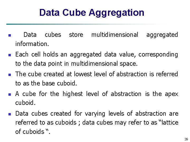
Data Cube Aggregation n n Data cubes information. store multidimensional aggregated Each cell holds an aggregated data value, corresponding to the data point in multidimensional space. The cube created at lowest level of abstraction is referred to as the base cuboid. A cube for the highest level of abstraction is the apex cuboid. Data cubes created for varying levels of abstraction are referred to as cuboids ; data cubes may refer to as “lattice of cuboids “. 39

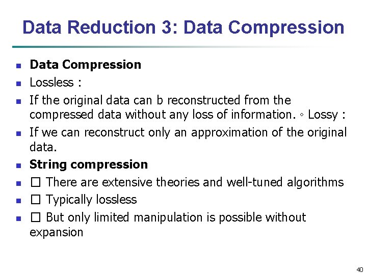
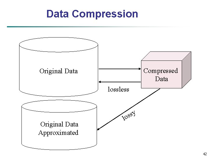
Data Reduction 3: Data Compression n n n n Data Compression Lossless : If the original data can b reconstructed from the compressed data without any loss of information. ◦ Lossy : If we can reconstruct only an approximation of the original data. String compression � There are extensive theories and well-tuned algorithms � Typically lossless � But only limited manipulation is possible without expansion 40

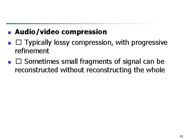
n n n Audio/video compression � Typically lossy compression, with progressive refinement � Sometimes small fragments of signal can be reconstructed without reconstructing the whole 41

Data Compression Compressed Data Original Data lossless Original Data Approximated y s s lo 42

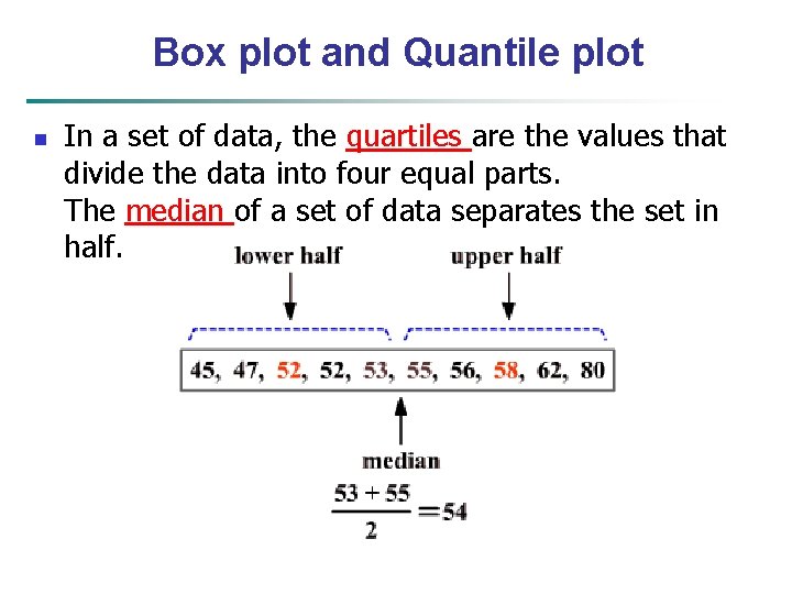
Box plot and Quantile plot n In a set of data, the quartiles are the values that divide the data into four equal parts. The median of a set of data separates the set in half.

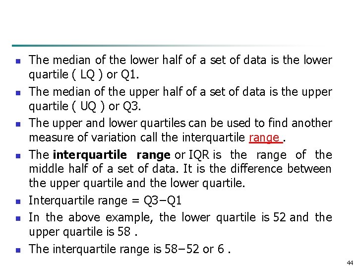
n n n n The median of the lower half of a set of data is the lower quartile ( LQ ) or Q 1. The median of the upper half of a set of data is the upper quartile ( UQ ) or Q 3. The upper and lower quartiles can be used to find another measure of variation call the interquartile range. The interquartile range or IQR is the range of the middle half of a set of data. It is the difference between the upper quartile and the lower quartile. Interquartile range = Q 3−Q 1 In the above example, the lower quartile is 52 and the upper quartile is 58. The interquartile range is 58− 52 or 6. 44

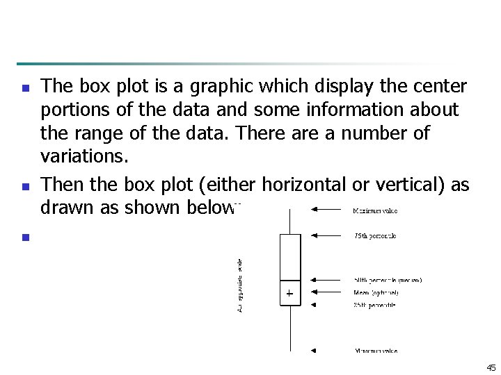
n n The box plot is a graphic which display the center portions of the data and some information about the range of the data. There a number of variations. Then the box plot (either horizontal or vertical) as drawn as shown below: n 45

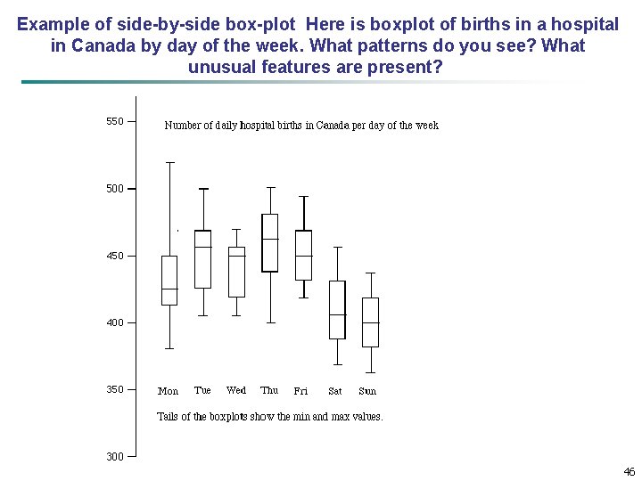
Example of side-by-side box-plot Here is boxplot of births in a hospital in Canada by day of the week. What patterns do you see? What unusual features are present? 46

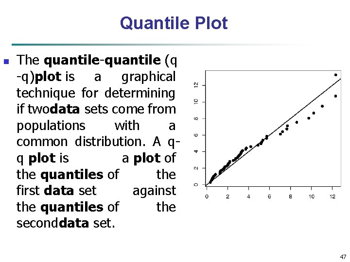
Quantile Plot n The quantile-quantile (q -q)plot is a graphical technique for determining if twodata sets come from populations with a common distribution. A qq plot is a plot of the quantiles of the first data set against the quantiles of the seconddata set. 47

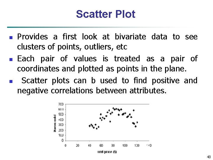
Scatter Plot n n n Provides a first look at bivariate data to see clusters of points, outliers, etc Each pair of values is treated as a pair of coordinates and plotted as points in the plane. Scatter plots can b used to find positive and negative correlations between attributes. 48

Chapter 3: Data Preprocessing n Data Preprocessing: An Overview n Data Quality n Major Tasks in Data Preprocessing n Data Cleaning n Data Integration n Data Reduction n Data Transformation and Data Discretization n Summary 49

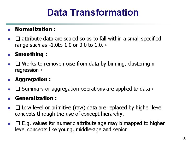
Data Transformation n n Normalization : � attribute data are scaled so as to fall within a small specified range such as -1. 0 to 1. 0 or 0. 0 to 1. 0. ◦ Smoothing : � Works to remove noise from data by binning, clustering n regression ◦ n Aggregation : n � Summary or aggregation operations are applied to data ◦ n Generalization : n n � Low level or primitive (raw) data are replaced by higher level concepts through the use of concept hierarchy. � E. g. values for numeric attribute age may b mapped to higher level concepts like young, middle-age and senior. 50

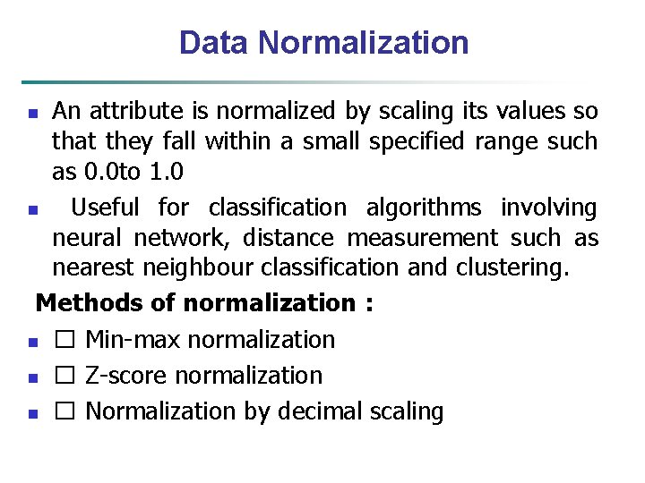
Data Normalization An attribute is normalized by scaling its values so that they fall within a small specified range such as 0. 0 to 1. 0 n Useful for classification algorithms involving neural network, distance measurement such as nearest neighbour classification and clustering. Methods of normalization : n � Min-max normalization n � Z-score normalization n � Normalization by decimal scaling n

Normalization n Min-max normalization: to [new_min. A, new_max. A] n n Z-score normalization (μ: mean, σ: standard deviation): n n Ex. Let income range $12, 000 to $98, 000 normalized to [0. 0, 1. 0]. Then $73, 000 is mapped to Ex. Let μ = 54, 000, σ = 16, 000. Then Normalization by decimal scaling Where j is the smallest integer such that Max(|ν’|) < 1 52

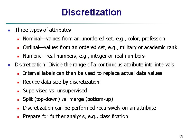
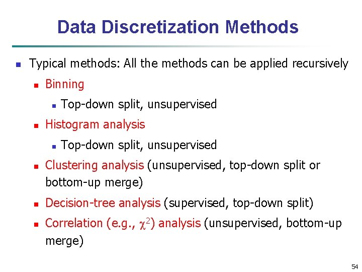
Discretization n n Three types of attributes n Nominal—values from an unordered set, e. g. , color, profession n Ordinal—values from an ordered set, e. g. , military or academic rank n Numeric—real numbers, e. g. , integer or real numbers Discretization: Divide the range of a continuous attribute into intervals n Interval labels can then be used to replace actual data values n Reduce data size by discretization n Supervised vs. unsupervised n Split (top-down) vs. merge (bottom-up) n Discretization can be performed recursively on an attribute n Prepare for further analysis, e. g. , classification 53

Data Discretization Methods n Typical methods: All the methods can be applied recursively n Binning n n Histogram analysis n n Top-down split, unsupervised Clustering analysis (unsupervised, top-down split or bottom-up merge) Decision-tree analysis (supervised, top-down split) Correlation (e. g. , 2) analysis (unsupervised, bottom-up merge) 54

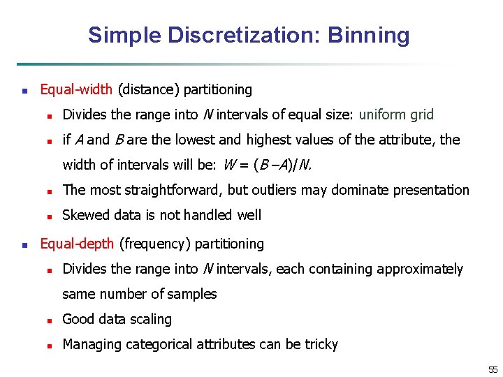
Simple Discretization: Binning n Equal-width (distance) partitioning n Divides the range into N intervals of equal size: uniform grid n if A and B are the lowest and highest values of the attribute, the width of intervals will be: W = (B –A)/N. n n The most straightforward, but outliers may dominate presentation n Skewed data is not handled well Equal-depth (frequency) partitioning n Divides the range into N intervals, each containing approximately same number of samples n Good data scaling n Managing categorical attributes can be tricky 55

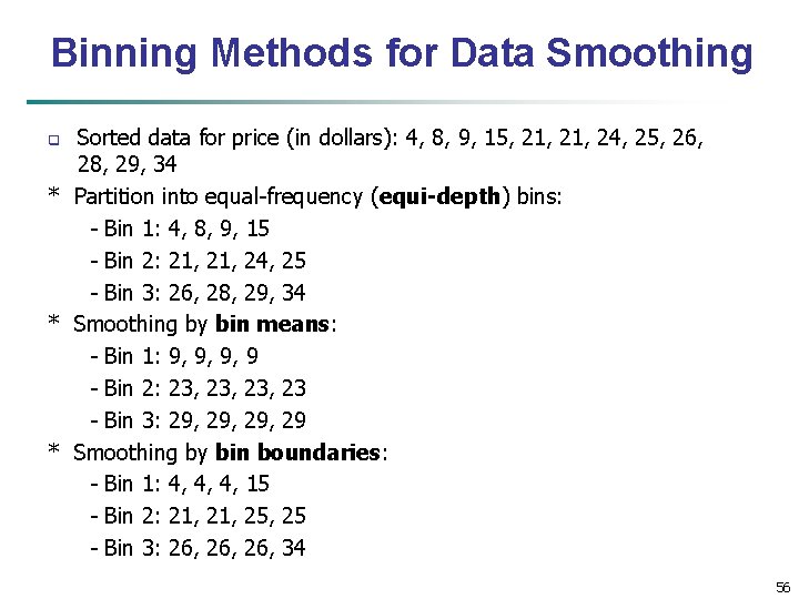
Binning Methods for Data Smoothing Sorted data for price (in dollars): 4, 8, 9, 15, 21, 24, 25, 26, 28, 29, 34 * Partition into equal-frequency (equi-depth) bins: - Bin 1: 4, 8, 9, 15 - Bin 2: 21, 24, 25 - Bin 3: 26, 28, 29, 34 * Smoothing by bin means: - Bin 1: 9, 9, 9, 9 - Bin 2: 23, 23, 23 - Bin 3: 29, 29, 29 * Smoothing by bin boundaries: - Bin 1: 4, 4, 4, 15 - Bin 2: 21, 25, 25 - Bin 3: 26, 26, 34 q 56

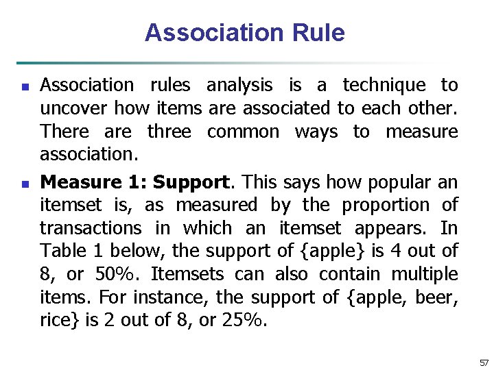
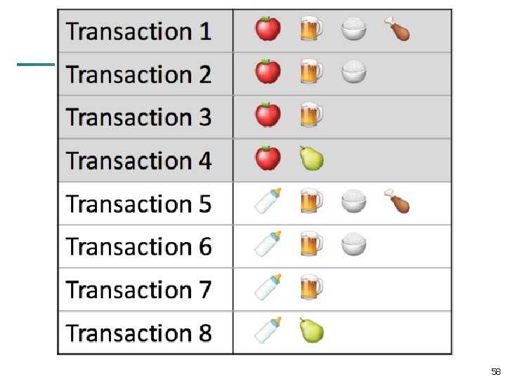
Association Rule n n Association rules analysis is a technique to uncover how items are associated to each other. There are three common ways to measure association. Measure 1: Support. This says how popular an itemset is, as measured by the proportion of transactions in which an itemset appears. In Table 1 below, the support of {apple} is 4 out of 8, or 50%. Itemsets can also contain multiple items. For instance, the support of {apple, beer, rice} is 2 out of 8, or 25%. 57

58

n If you discover that sales of items beyond a certain proportion tend to have a significant impact on your profits, you might consider using that proportion as your support threshold. You may then identify itemsets with support values above this threshold as significant itemsets. 59

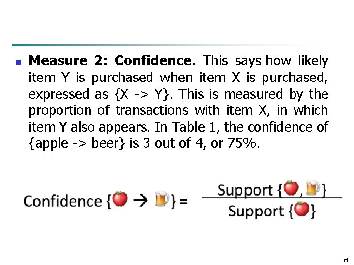
n Measure 2: Confidence. This says how likely item Y is purchased when item X is purchased, expressed as {X -> Y}. This is measured by the proportion of transactions with item X, in which item Y also appears. In Table 1, the confidence of {apple -> beer} is 3 out of 4, or 75%. 60

n One drawback of the confidence measure is that it might misrepresent the importance of an association. This is because it only accounts for how popular apples are, but not beers. If beers are also very popular in general, there will be a higher chance that a transaction containing apples will also contain beers, thus inflating the confidence measure. 61

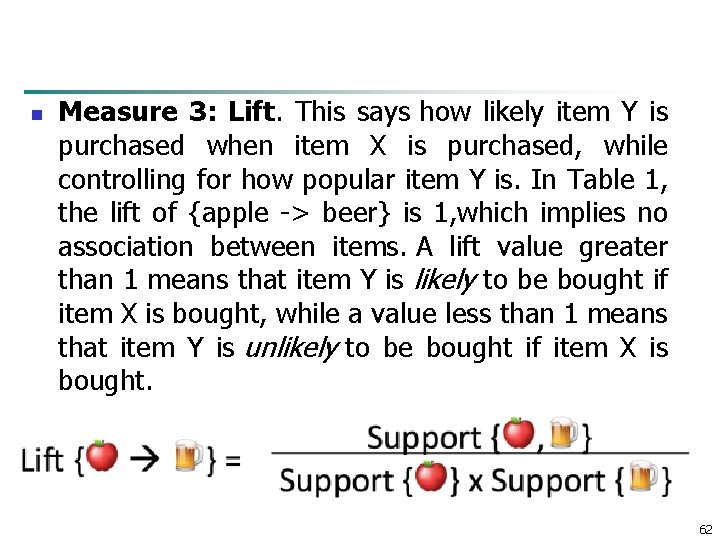
n Measure 3: Lift. This says how likely item Y is purchased when item X is purchased, while controlling for how popular item Y is. In Table 1, the lift of {apple -> beer} is 1, which implies no association between items. A lift value greater than 1 means that item Y is likely to be bought if item X is bought, while a value less than 1 means that item Y is unlikely to be bought if item X is bought. 62

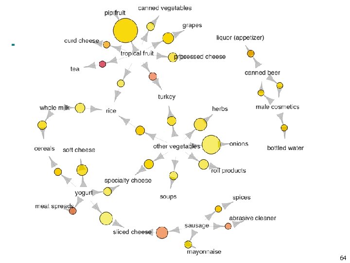
n We use a dataset on grocery transactions from the arules R library. It contains actual transactions at a grocery outlet over 30 days. The network graph below shows associations between selected items. Larger circles imply higher support, while red circles imply higher lift: 63

64

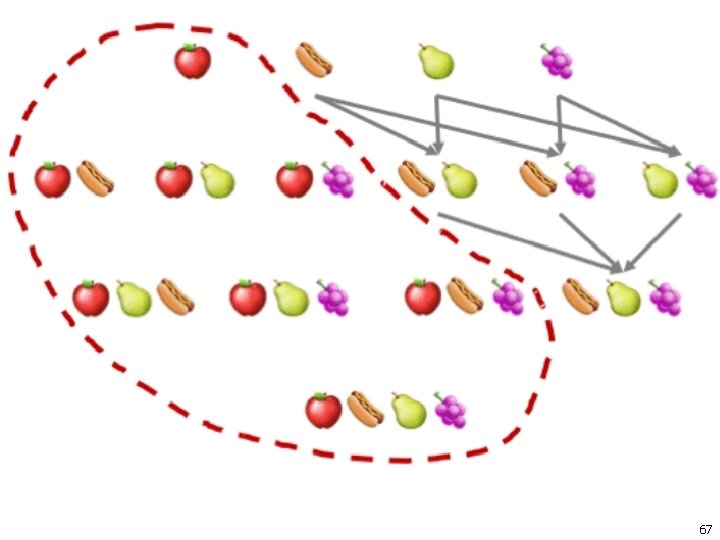
Apriori Algorithm n n n The apriori principle can reduce the number of itemsets we need to examine. Put simply, the apriori principle states that if an itemset is infrequent, then all its supersets must also be infrequent This means that if {beer} was found to be infrequent, we can expect {beer, pizza} to be equally or even more infrequent. So in consolidating the list of popular itemsets, we need not consider {beer, pizza}, nor any other itemset configuration that contains beer. 65

Finding itemsets with high support n n n Using the apriori principle, the number of itemsets that have to be examined can be pruned, and the list of popular itemsets can be obtained in these steps: Step 0. Start with itemsets containing just a single item, such as {apple} and {pear}. Step 1. Determine the support for itemsets. Keep the itemsets that meet your minimum support threshold, and remove itemsets that do not. Step 2. Using the itemsets you have kept from Step 1, generate all the possible itemset configurations. Step 3. Repeat Steps 1 & 2 until there are no more new itemsets. 66

67

n n What is the use of learning association rules? Shopping centers use association rules to place the items next to each other so that users buy more items. If you are familiar with data mining you would know about the famous beer-diapers-Wal-Mart story. Basically Wal-Mart studied their data and found that on Friday afternoon young American males who buy diapers also tend to buy beer. So Wal-Mart placed beer next to diapers and the beer-sales went up. This is famous because no one would have predicted such a result and that’s the power of data mining. You can Google for this if you are interested in further details Also if you are familiar with Amazon, they use association mining to recommend you the items based on the current item you are browsing/buying. Another application is the Google auto-complete, where after you type in a word it searches frequently associated words that user type after that particular word. 68

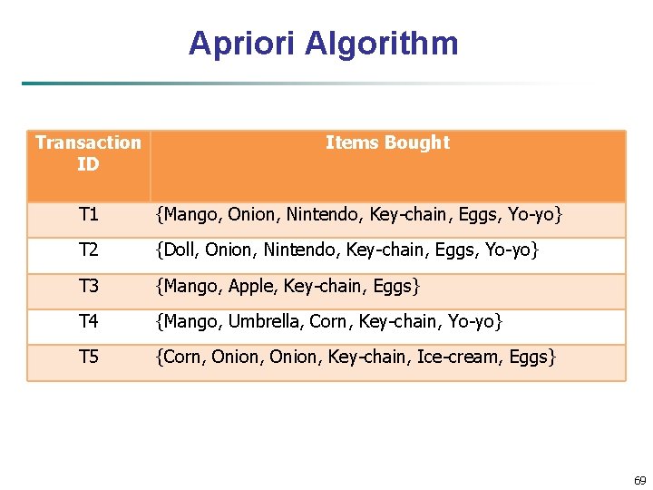
Apriori Algorithm Transaction ID Items Bought T 1 {Mango, Onion, Nintendo, Key-chain, Eggs, Yo-yo} T 2 {Doll, Onion, Nintendo, Key-chain, Eggs, Yo-yo} T 3 {Mango, Apple, Key-chain, Eggs} T 4 {Mango, Umbrella, Corn, Key-chain, Yo-yo} T 5 {Corn, Onion, Key-chain, Ice-cream, Eggs} 69

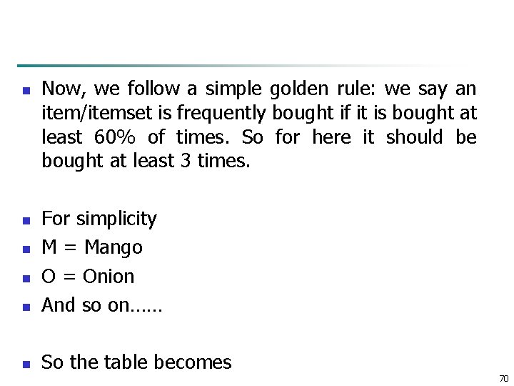
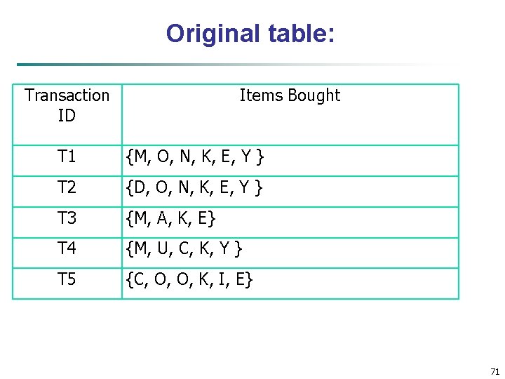
n Now, we follow a simple golden rule: we say an item/itemset is frequently bought if it is bought at least 60% of times. So for here it should be bought at least 3 times. n For simplicity M = Mango O = Onion And so on…… n So the table becomes n n n 70

Original table: Transaction ID Items Bought T 1 {M, O, N, K, E, Y } T 2 {D, O, N, K, E, Y } T 3 {M, A, K, E} T 4 {M, U, C, K, Y } T 5 {C, O, O, K, I, E} 71

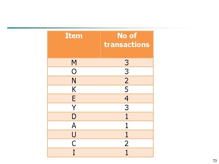
n Step 1: Count the number of transactions in which each item occurs, Note ‘O=Onion’ is bought 4 times in total, but, it occurs in just 3 transactions. 72

Item No of transactions M O N K E Y D A U C I 3 3 2 5 4 3 1 1 1 2 1 73

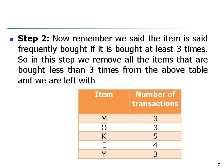
n Step 2: Now remember we said the item is said frequently bought if it is bought at least 3 times. So in this step we remove all the items that are bought less than 3 times from the above table and we are left with Item Number of transactions M O K E Y 3 3 5 4 3 74

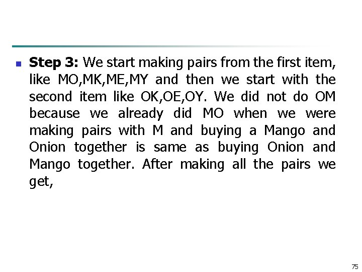
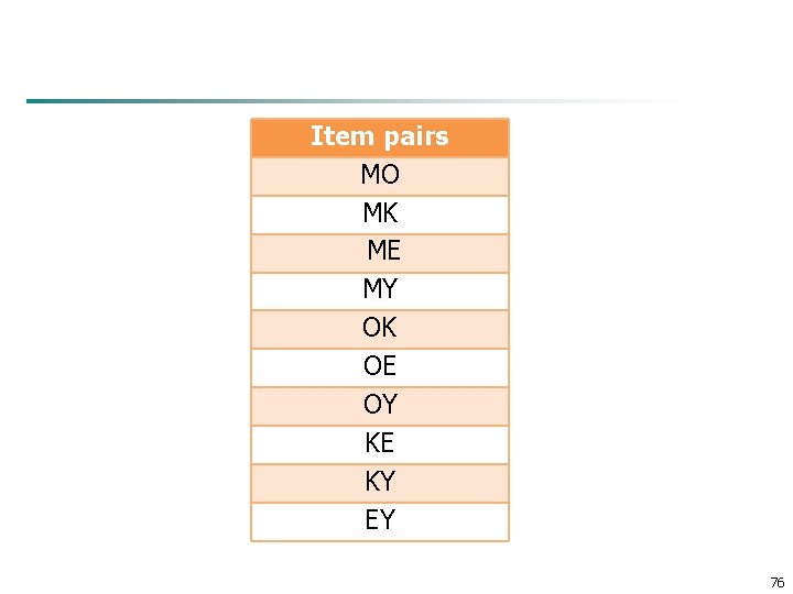
n Step 3: We start making pairs from the first item, like MO, MK, ME, MY and then we start with the second item like OK, OE, OY. We did not do OM because we already did MO when we were making pairs with M and buying a Mango and Onion together is same as buying Onion and Mango together. After making all the pairs we get, 75

Item pairs MO MK ME MY OK OE OY KE KY EY 76

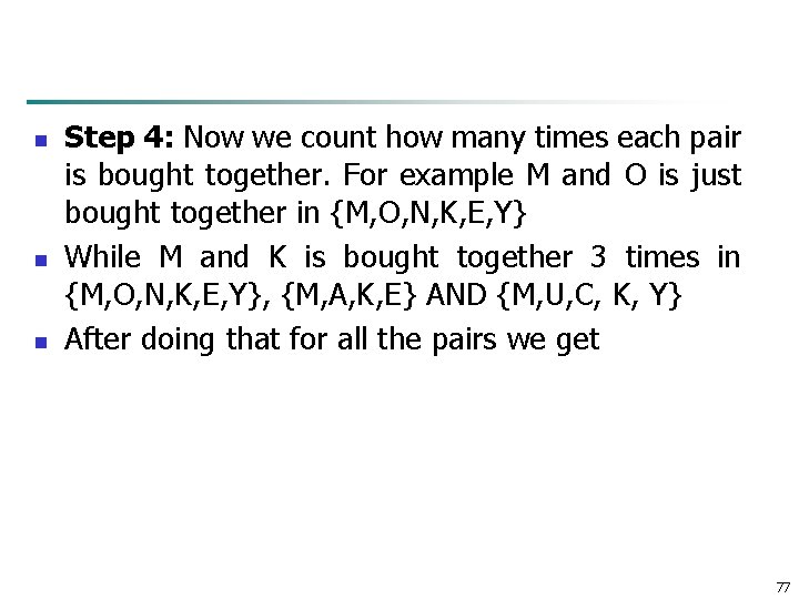
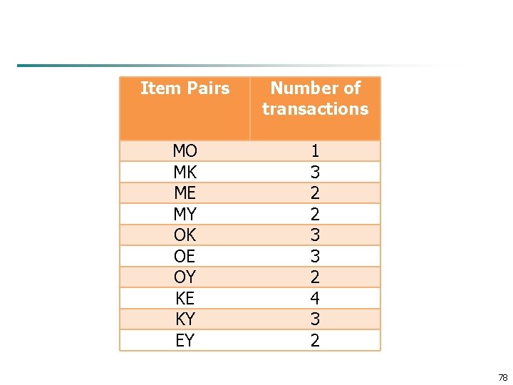
n n n Step 4: Now we count how many times each pair is bought together. For example M and O is just bought together in {M, O, N, K, E, Y} While M and K is bought together 3 times in {M, O, N, K, E, Y}, {M, A, K, E} AND {M, U, C, K, Y} After doing that for all the pairs we get 77

Item Pairs Number of transactions MO MK ME MY OK OE OY KE KY EY 1 3 2 2 3 3 2 4 3 2 78

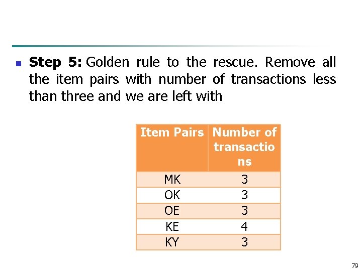
n Step 5: Golden rule to the rescue. Remove all the item pairs with number of transactions less than three and we are left with Item Pairs Number of transactio ns MK OK OE KE KY 3 3 3 4 3 79

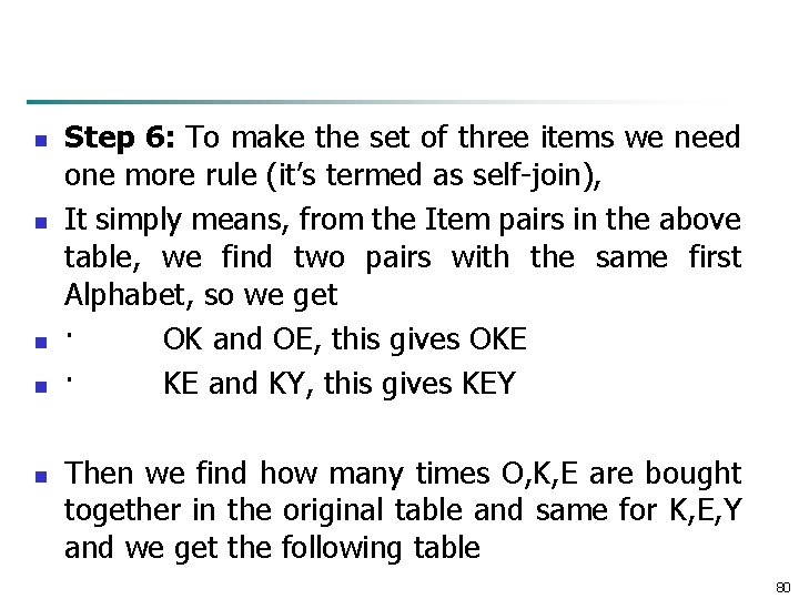
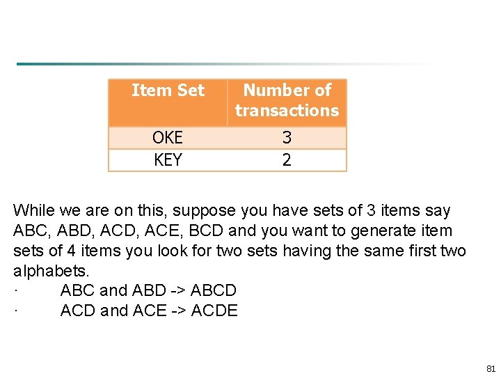
n n n Step 6: To make the set of three items we need one more rule (it’s termed as self-join), It simply means, from the Item pairs in the above table, we find two pairs with the same first Alphabet, so we get · OK and OE, this gives OKE · KE and KY, this gives KEY Then we find how many times O, K, E are bought together in the original table and same for K, E, Y and we get the following table 80

Item Set Number of transactions OKE KEY 3 2 While we are on this, suppose you have sets of 3 items say ABC, ABD, ACE, BCD and you want to generate item sets of 4 items you look for two sets having the same first two alphabets. · ABC and ABD -> ABCD · ACD and ACE -> ACDE 81