Structure and function of nucleic acids DNA structure

Structure and function of nucleic acids.

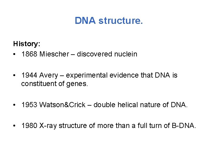
DNA structure. History: • 1868 Miescher – discovered nuclein • 1944 Avery – experimental evidence that DNA is constituent of genes. • 1953 Watson&Crick – double helical nature of DNA. • 1980 X-ray structure of more than a full turn of B-DNA.

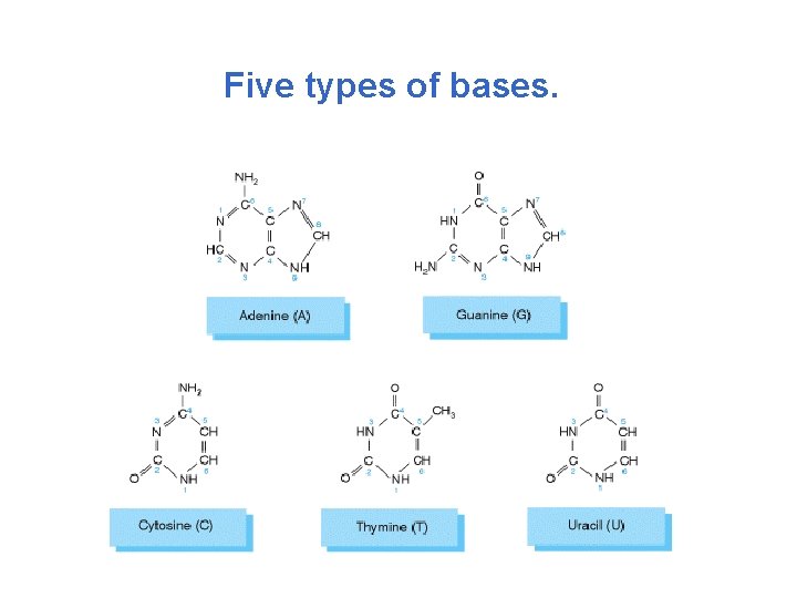
Five types of bases.

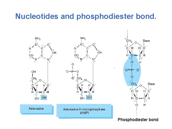
Nucleotides and phosphodiester bond. Phosphodiester bond

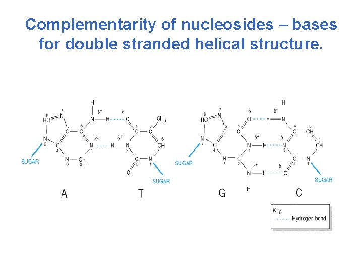
Complementarity of nucleosides – bases for double stranded helical structure.

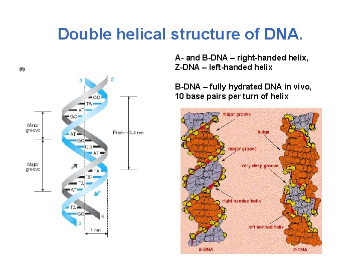
Double helical structure of DNA. A- and B-DNA – right-handed helix, Z-DNA – left-handed helix B-DNA – fully hydrated DNA in vivo, 10 base pairs per turn of helix

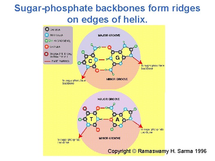
Sugar-phosphate backbones form ridges on edges of helix. Copyright © Ramaswamy H. Sarma 1996

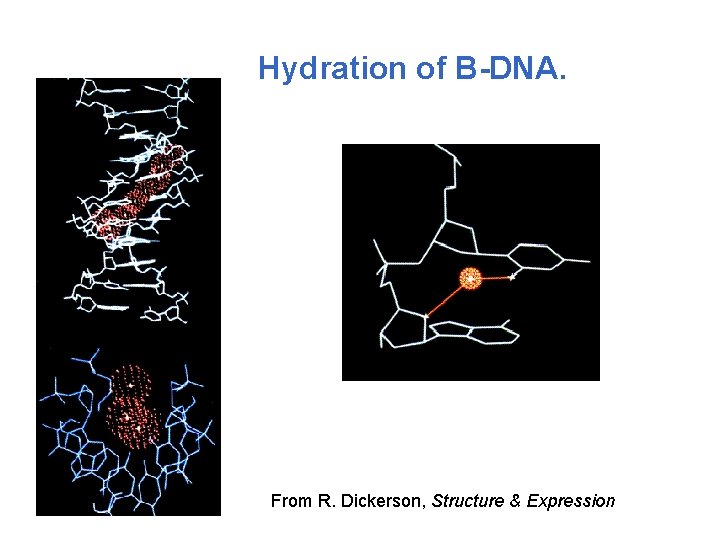
Hydration of B-DNA. From R. Dickerson, Structure & Expression

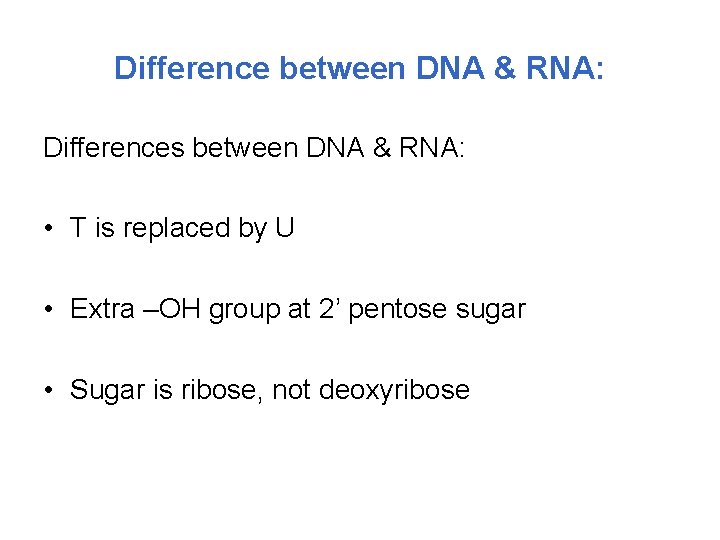
Difference between DNA & RNA: Differences between DNA & RNA: • T is replaced by U • Extra –OH group at 2’ pentose sugar • Sugar is ribose, not deoxyribose

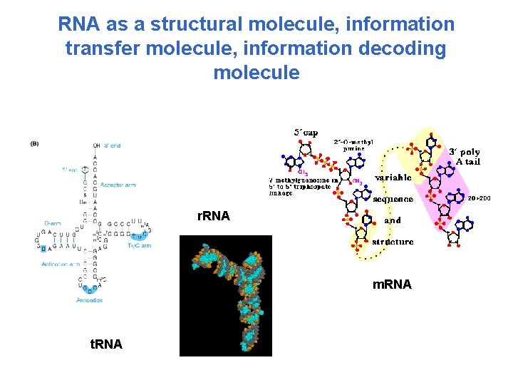
RNA as a structural molecule, information transfer molecule, information decoding molecule r. RNA m. RNA t. RNA

Classwork I. 1. Go to http: //ndbserver. rutgers. edu/. 2. Select Crystal structure of B-DNA, resolution >=2 Angstroms. 3. Select Crystal structure of single-stranded RNA with mismatch base pairing with resolution >= 2 Angstroms.

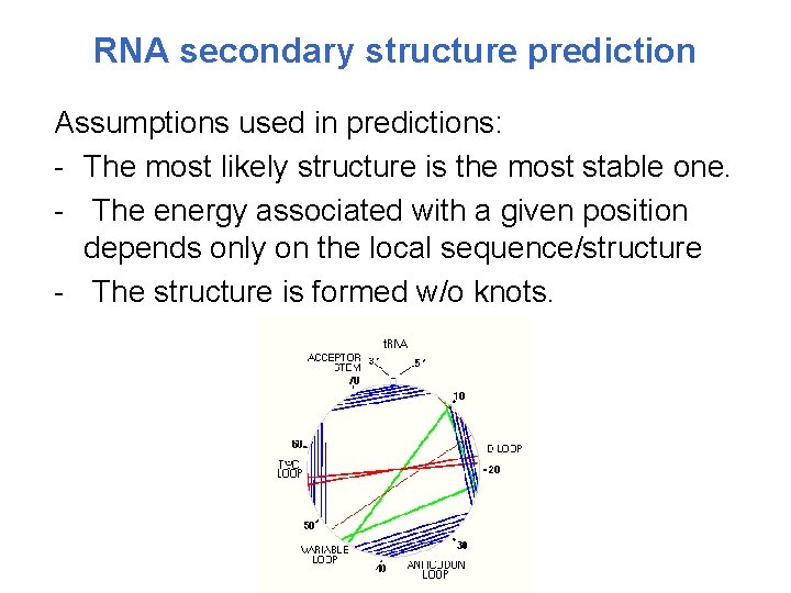
RNA secondary structure prediction Assumptions used in predictions: - The most likely structure is the most stable one. - The energy associated with a given position depends only on the local sequence/structure - The structure is formed w/o knots.

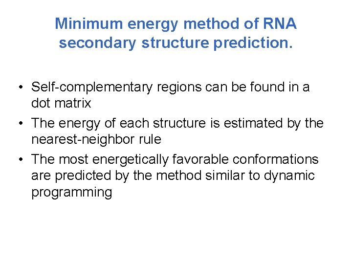
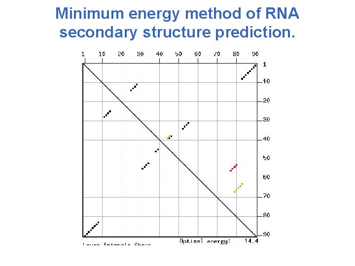
Minimum energy method of RNA secondary structure prediction. • Self-complementary regions can be found in a dot matrix • The energy of each structure is estimated by the nearest-neighbor rule • The most energetically favorable conformations are predicted by the method similar to dynamic programming

Minimum energy method of RNA secondary structure prediction.

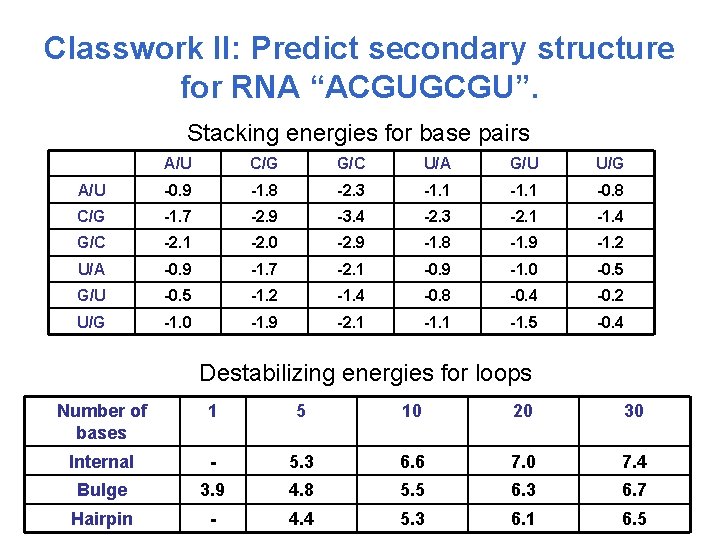
Classwork II: Predict secondary structure for RNA “ACGUGCGU”. Stacking energies for base pairs A/U C/G G/C U/A G/U U/G A/U -0. 9 -1. 8 -2. 3 -1. 1 -0. 8 C/G -1. 7 -2. 9 -3. 4 -2. 3 -2. 1 -1. 4 G/C -2. 1 -2. 0 -2. 9 -1. 8 -1. 9 -1. 2 U/A -0. 9 -1. 7 -2. 1 -0. 9 -1. 0 -0. 5 G/U -0. 5 -1. 2 -1. 4 -0. 8 -0. 4 -0. 2 U/G -1. 0 -1. 9 -2. 1 -1. 5 -0. 4 Destabilizing energies for loops Number of bases 1 5 10 20 30 Internal - 5. 3 6. 6 7. 0 7. 4 Bulge 3. 9 4. 8 5. 5 6. 3 6. 7 Hairpin - 4. 4 5. 3 6. 1 6. 5

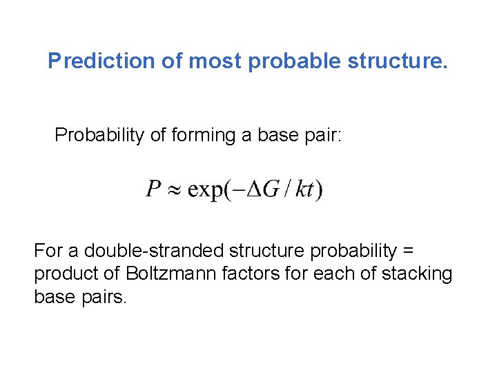
Prediction of most probable structure. Probability of forming a base pair: For a double-stranded structure probability = product of Boltzmann factors for each of stacking base pairs.

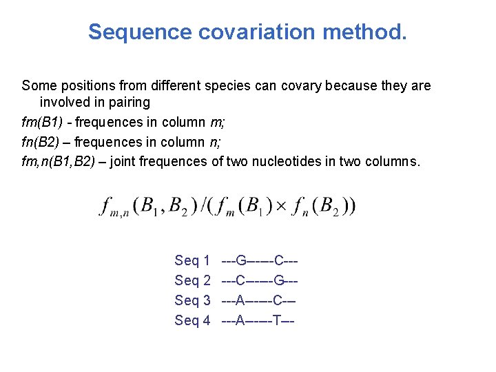
Sequence covariation method. Some positions from different species can covary because they are involved in pairing fm(B 1) - frequences in column m; fn(B 2) – frequences in column n; fm, n(B 1, B 2) – joint frequences of two nucleotides in two columns. Seq 1 Seq 2 Seq 3 Seq 4 ---G------C------G-----A------C-----A------T---

Ribozymes. • RNA of self-splicing group I introns, contain 4 sequence elements and form specific secondary structures • RNA self-splicing group II introns • RNA from viral and plant satellite RNAs • Ribosomal RNAs

Gene prediction. Gene – DNA sequence encoding protein, r. RNA, t. RNA (sn. RNA, sno. RNA)… Gene concept is complicated: - Introns/exons - Alternative splicing - Genes-in-genes - Multisubunit proteins

Gene identification • Homology-based gene prediction – Similarity Searches (e. g. BLAST, BLAT) – Genome Browsers – RNA evidence (ESTs) • Ab initio gene prediction – Prokaryotes • ORF identification – Eukaryotes • Promoter prediction • Poly. A-signal prediction • Splice site, start/stop-codon predictions

Prokaryotic genes – searching for ORFs. - Small genomes have high gene density Haemophilus influenza – 85% genic - No introns - Operons One transcript, many genes - Open reading frames (ORF) – contiguous set of codons, start with Met-codon, ends with stop codon.

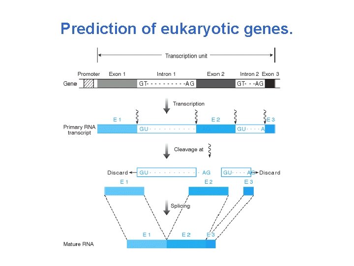
Prediction of eukaryotic genes.

Ab initio gene prediction. Predictions are based on the observation that gene DNA sequence is not random: - Each species has a characteristic pattern of synonymous codon usage. - Every third base tends to be the same. - Non-coding ORFs are very short. Gene. Mark (HMMs), Gen. Scan, Grail II(neural networks) and Gene. Parser (DP)

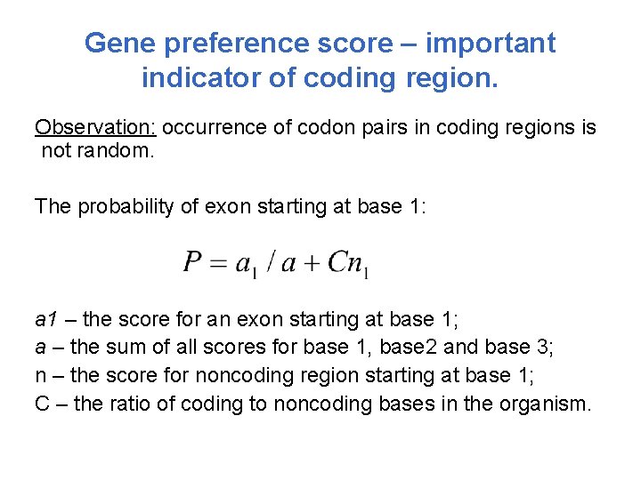
Gene preference score – important indicator of coding region. Observation: occurrence of codon pairs in coding regions is not random. The probability of exon starting at base 1: a 1 – the score for an exon starting at base 1; a – the sum of all scores for base 1, base 2 and base 3; n – the score for noncoding region starting at base 1; C – the ratio of coding to noncoding bases in the organism.

Confirming gene location using EST libraries. • Expressed Sequence Tags (ESTs) – sequenced short segments of c. DNA. They are organized in the database “Uni. Gene”. • If region matches ESTs with high statistical significance, then it is a gene or pseudogene.

Gene prediction accuracy. Factors which influence the accuracy: - genetic code of a given genome may differ from the universal code - one tissue can splice one m. RNA differently from another - m. RNA can be edited

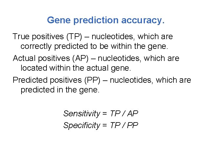
Gene prediction accuracy. True positives (TP) – nucleotides, which are correctly predicted to be within the gene. Actual positives (AP) – nucleotides, which are located within the actual gene. Predicted positives (PP) – nucleotides, which are predicted in the gene. Sensitivity = TP / AP Specificity = TP / PP

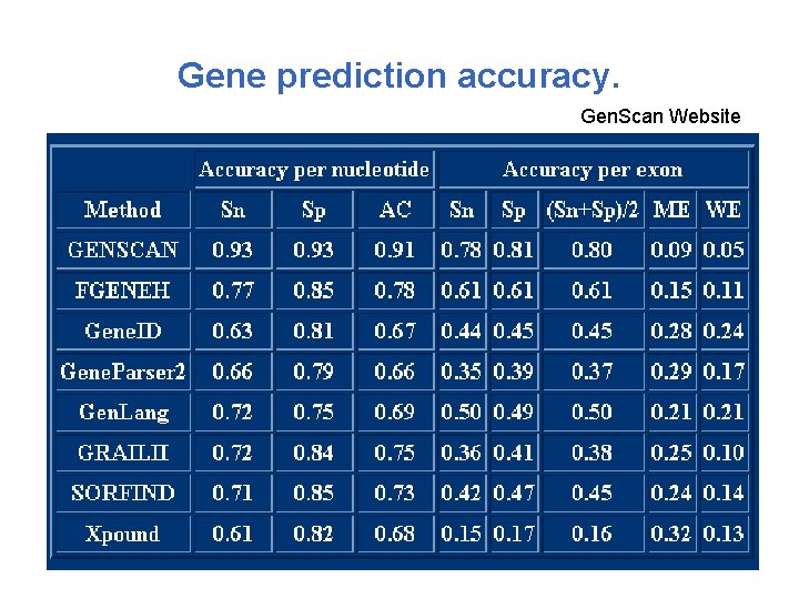
Gene prediction accuracy. Gen. Scan Website

Common difficulties • First and last exons difficult to annotate because they contain UTRs. • Smaller genes are not statistically significant so they are thrown out. • Algorithms are trained with sequences from known genes which biases them against genes about which nothing is known.

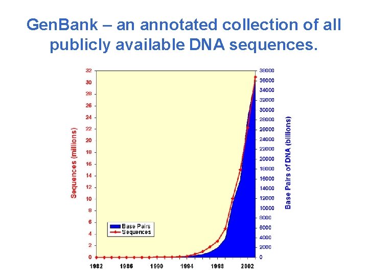
Gen. Bank – an annotated collection of all publicly available DNA sequences.

Gene prediction: classwork III. • Go to http: //www. ncbi. nlm. nih. gov/mapview/ and view all hemoglobin genes of H. sapiens • Find 6 hemoglobin genes on chromosome 11, view the DNA sequence of this chromosome region • Submit this sequence to Gen. Scan server at http: //genes. mit. edu/GENSCAN. html

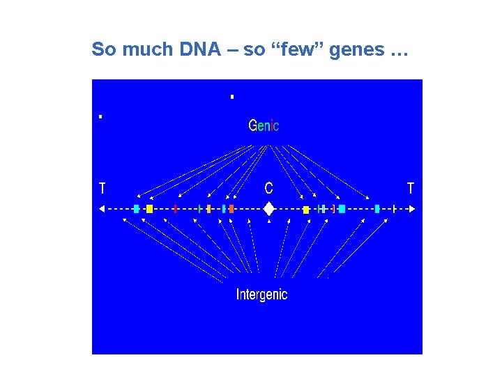
Genome analysis. Genome – the sum of genes and intergenic sequences of haploid cell.

The value of genome sequences lies in their annotation • Annotation – Characterizing genomic features using computational and experimental methods • Genes: Four levels of annotation – Gene Prediction – Where are genes? – What do they look like? – What do they encode? – What proteins/pathways involved in?

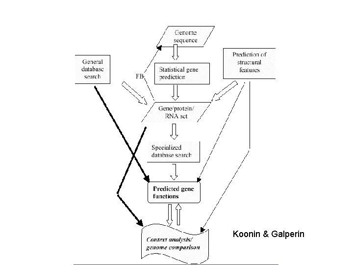
Koonin & Galperin

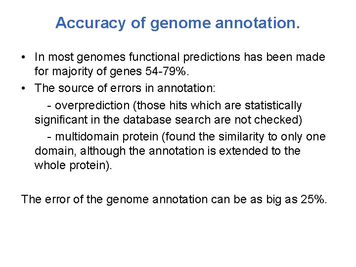
Accuracy of genome annotation. • In most genomes functional predictions has been made for majority of genes 54 -79%. • The source of errors in annotation: - overprediction (those hits which are statistically significant in the database search are not checked) - multidomain protein (found the similarity to only one domain, although the annotation is extended to the whole protein). The error of the genome annotation can be as big as 25%.

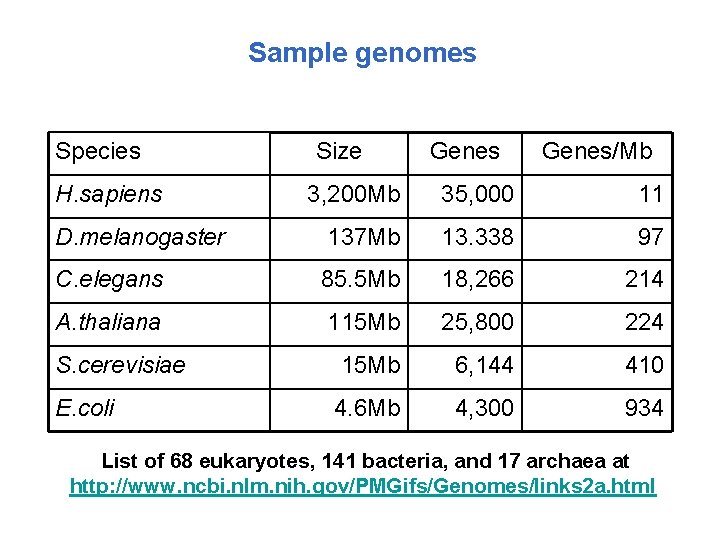
Sample genomes Species H. sapiens Size Genes/Mb 3, 200 Mb 35, 000 11 D. melanogaster 137 Mb 13. 338 97 C. elegans 85. 5 Mb 18, 266 214 A. thaliana 115 Mb 25, 800 224 S. cerevisiae 15 Mb 6, 144 410 E. coli 4. 6 Mb 4, 300 934 List of 68 eukaryotes, 141 bacteria, and 17 archaea at http: //www. ncbi. nlm. nih. gov/PMGifs/Genomes/links 2 a. html

So much DNA – so “few” genes …

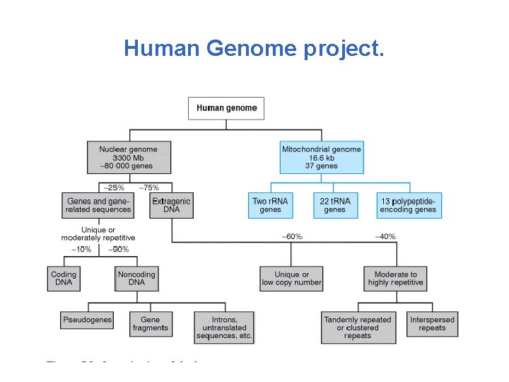
Human Genome project.

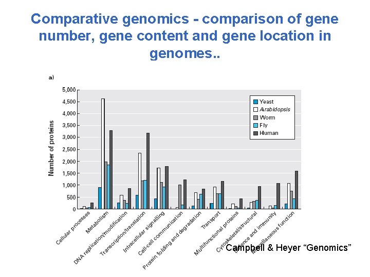
Comparative genomics - comparison of gene number, gene content and gene location in genomes. . Campbell & Heyer “Genomics”

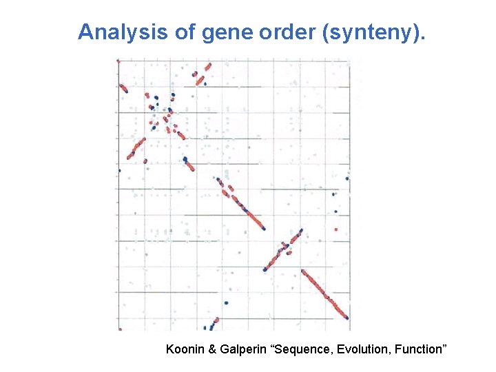
Analysis of gene order (synteny). Genes with a related function are frequently clustered on the chromosome. Ex: E. coli genes responsible for synthesis of Trp are clustered and order is conserved between different bacterial species. Operon: set of genes transcribed simultaneously with the same direction of transcription

Analysis of gene order (synteny). Koonin & Galperin “Sequence, Evolution, Function”

Analysis of gene order (synteny). • The order of genes is not very well conserved if %identity between prokaryotic genomes is < 50% • The gene neighborhood can be conserved so that the all neighboring genes belong to the same functional class. • Functional prediction based on gene neighboring.

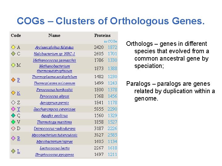
COGs – Clusters of Orthologous Genes. Orthologs – genes in different species that evolved from a common ancestral gene by speciation; Paralogs – paralogs are genes related by duplication within a genome.