Stereology 27 750 Texture Microstructure Anisotropy A D

Stereology 27 -750 Texture, Microstructure & Anisotropy A. D. Rollett Last revised: 24 th March 2016

2 Outline • Objectives • Motivation • Quantities, – definitions – measurable – Derivable • Problems that use Stereology, Topology • Volume fractions • Surface area per unit volume • Facet areas • Oriented objects • Particle spacings – Mean Free Path – Nearest Neighbor Distance • Zener Pinning • Grain Size • Sections through objects – Size Distributions

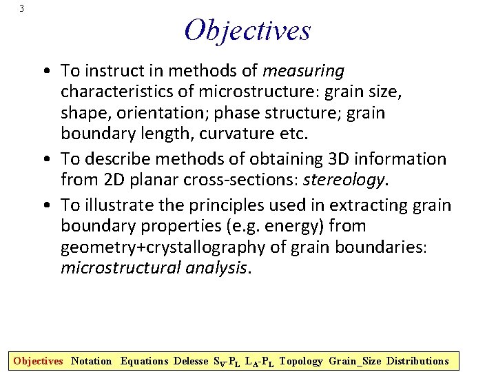
3 Objectives • To instruct in methods of measuring characteristics of microstructure: grain size, shape, orientation; phase structure; grain boundary length, curvature etc. • To describe methods of obtaining 3 D information from 2 D planar cross-sections: stereology. • To illustrate the principles used in extracting grain boundary properties (e. g. energy) from geometry+crystallography of grain boundaries: microstructural analysis. Objectives Notation Equations Delesse SV-PL LA-PL Topology Grain_Size Distributions

4 Objectives, contd. • [Stereology] To show to obtain useful microstructural quantities from plane sections through microstructures. • [Image Analysis] To show one can analyze images to obtain data required for stereological analysis. • [Property Measurement] To illustrate the value of stereological methods for obtaining relative interfacial energies from measurements of relative frequency of faceted particles. • Note that true 3 D data is available from serial sectioning, tomography, and 3 D microscopy (using diffraction). All these methods are time consuming and therefore it is always useful to be able to infer 3 D information from standard 2 D sections. Objectives Notation Equations Delesse SV-PL LA-PL Topology Grain_Size Distributions

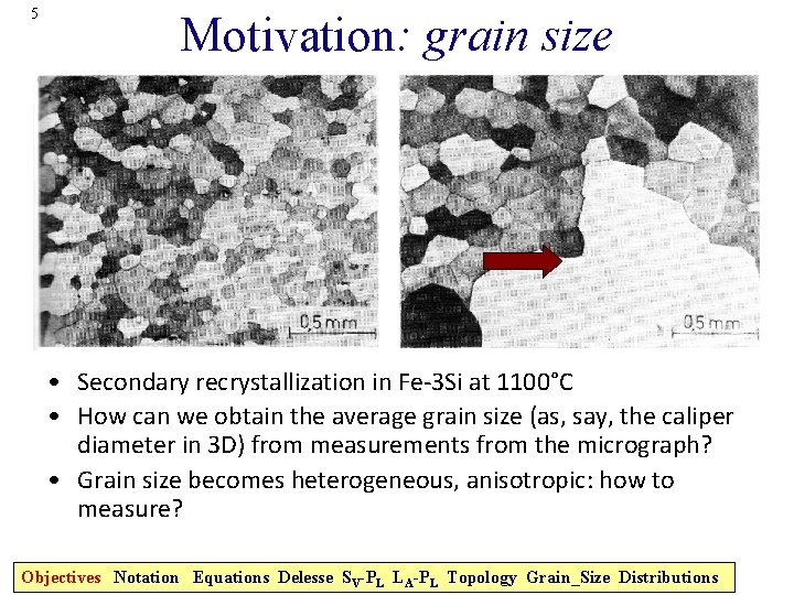
5 Motivation: grain size • Secondary recrystallization in Fe-3 Si at 1100°C • How can we obtain the average grain size (as, say, the caliper diameter in 3 D) from measurements from the micrograph? • Grain size becomes heterogeneous, anisotropic: how to measure? Objectives Notation Equations Delesse SV-PL LA-PL Topology Grain_Size Distributions

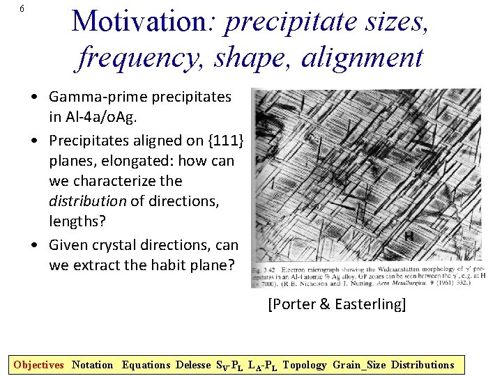
6 Motivation: precipitate sizes, frequency, shape, alignment • Gamma-prime precipitates in Al-4 a/o. Ag. • Precipitates aligned on {111} planes, elongated: how can we characterize the distribution of directions, lengths? • Given crystal directions, can we extract the habit plane? [Porter & Easterling] Objectives Notation Equations Delesse SV-PL LA-PL Topology Grain_Size Distributions

7 Stereology: References • • • • These slides are based on: Quantitative Stereology, E. E. Underwood, Addison-Wesley, 1970. - equation numbers given where appropriate. Practical Stereology, John Russ, Plenum (1986, IDBN 0 -306 -42460 -6). A very useful, open source software package for image analysis: Image. J, http: //rsb. info. nih. gov/ij/. A more comprehensive commercial image analysis software is Fovea. Pro, http: //www. reindeergraphics. com. Also useful, and more rigorous: M. G. Kendall & P. A. P. Moran, Geometrical Probability, Griffin (1963). More modern textbook, more mathematical in approach: Statistical Analysis of Microstructures in Materials Science, J. Ohser and F. Mücklich, Wiley, (2000, ISBN 0 -471 -97486 -2). Stereometric Metallography, S. A. Saltykov, Moscow: Metallurgizdat, 1958. Many practical (biological) examples of stereological measurement can be found in Unbiased Stereology, C. V. Howard & M. G. Reed, Springer (1998, ISBN 0 -387 -91516 -8). Random Heterogeneous Materials: Microstructure and Macroscopic Properties, S. Torquato, Springer Verlag (2001, ISBN 0 -387 -95167 -9). D. Sahagian and A. Proussevitch (1998) 3 D particle size distributions from 2 D observations: Stereology for natural applications, J Volcanol Geotherm Res, 84(3 -4), 173 -196. A. Brahme, M. H. Alvi, D. Saylor, J. Fridy, A. D. Rollett (2006) 3 D reconstruction of microstructure in a commercial purity aluminum, Scripta mater. 55(1): 75 -80. A. D. Rollett, R. Campman, D. Saylor (2006), Three dimensional microstructures: Statistical analysis of second phase particles in AA 7075 -T 651, Materials Science Forum 519 -521: 1 -10 Part 1 -2, Proceedings of the International Conference on Aluminium Alloys (ICAA-10), Vancouver, Canada. A. D. Rollett, S. -B. Lee, R. Campman and G. S. Rohrer, “Three-Dimensional Characterization of Microstructure by Electron Back-Scatter Diffraction, ” Annual Reviews in Materials Science, 37: 627 -658 (2007). M. A. Przystupa (1997) Estimation of true size distribution of partially aligned same-shape ellipsoidal particles, Scripta Mater. , 37(11), 1701 -1707. D. M. Saylor, J. Fridy, B El-Dasher, K. Jung, and A. D. Rollett (2004) Statistically Representative Three-Dimensional Microstructures Based on Orthogonal Observation Sections, Metall. Trans. A, 35 A, 1969 -1979. Objectives Notation Equations Delesse SV-PL LA-PL Topology Grain_Size Distributions

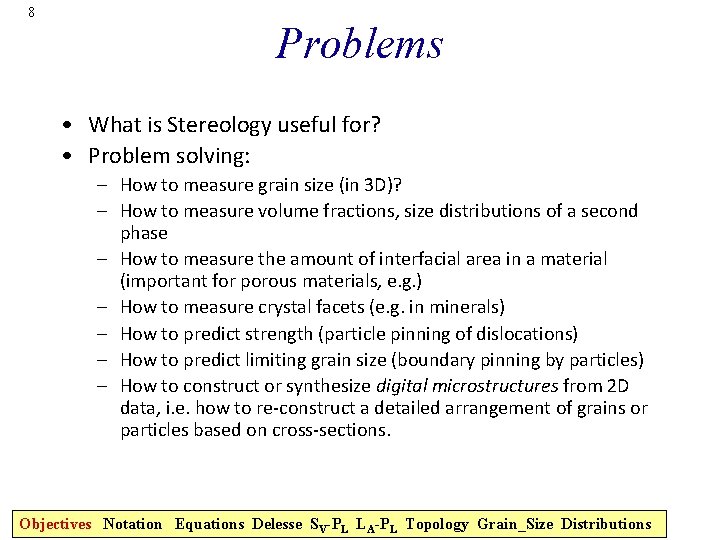
8 Problems • What is Stereology useful for? • Problem solving: – How to measure grain size (in 3 D)? – How to measure volume fractions, size distributions of a second phase – How to measure the amount of interfacial area in a material (important for porous materials, e. g. ) – How to measure crystal facets (e. g. in minerals) – How to predict strength (particle pinning of dislocations) – How to predict limiting grain size (boundary pinning by particles) – How to construct or synthesize digital microstructures from 2 D data, i. e. how to re-construct a detailed arrangement of grains or particles based on cross-sections. Objectives Notation Equations Delesse SV-PL LA-PL Topology Grain_Size Distributions

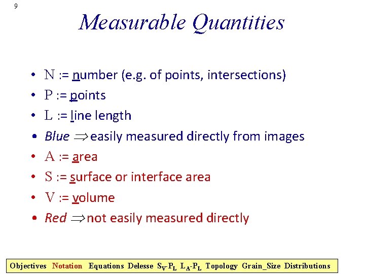
9 Measurable Quantities • • N : = number (e. g. of points, intersections) P : = points L : = line length Blue easily measured directly from images A : = area S : = surface or interface area V : = volume Red not easily measured directly Objectives Notation Equations Delesse SV-PL LA-PL Topology Grain_Size Distributions

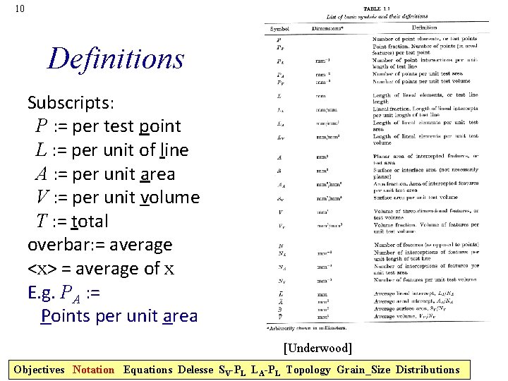
10 Definitions Subscripts: P : = per test point L : = per unit of line A : = per unit area V : = per unit volume T : = total overbar: = average <x> = average of x E. g. PA : = Points per unit area [Underwood] Objectives Notation Equations Delesse SV-PL LA-PL Topology Grain_Size Distributions

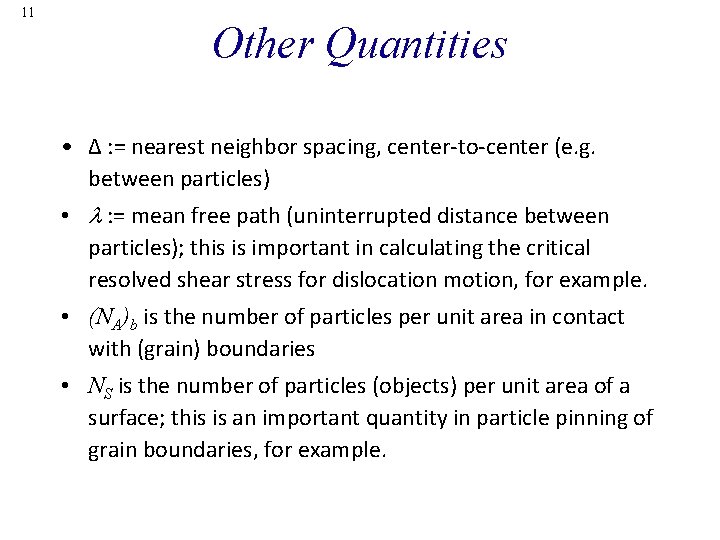
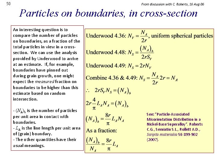
11 Other Quantities • ∆ : = nearest neighbor spacing, center-to-center (e. g. between particles) • : = mean free path (uninterrupted distance between particles); this is important in calculating the critical resolved shear stress for dislocation motion, for example. • (NA)b is the number of particles per unit area in contact with (grain) boundaries • NS is the number of particles (objects) per unit area of a surface; this is an important quantity in particle pinning of grain boundaries, for example.

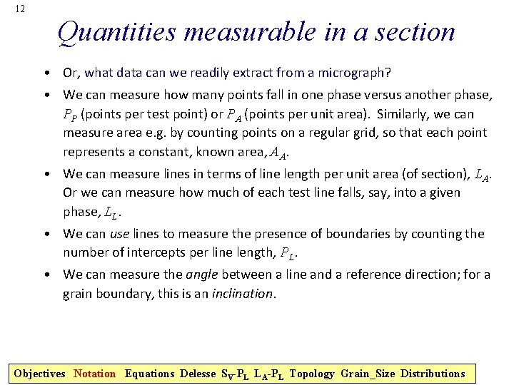
12 Quantities measurable in a section • Or, what data can we readily extract from a micrograph? • We can measure how many points fall in one phase versus another phase, PP (points per test point) or PA (points per unit area). Similarly, we can measure area e. g. by counting points on a regular grid, so that each point represents a constant, known area, AA. • We can measure lines in terms of line length per unit area (of section), LA. Or we can measure how much of each test line falls, say, into a given phase, LL. • We can use lines to measure the presence of boundaries by counting the number of intercepts per line length, PL. • We can measure the angle between a line and a reference direction; for a grain boundary, this is an inclination. Objectives Notation Equations Delesse SV-PL LA-PL Topology Grain_Size Distributions

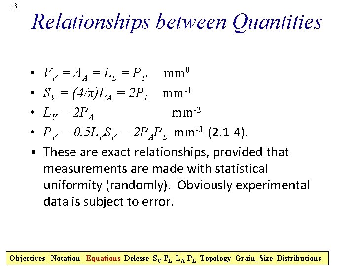
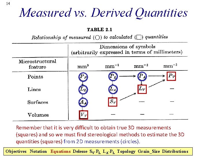
13 Relationships between Quantities • • • VV = AA = LL = PP mm 0 SV = (4/π)LA = 2 PL mm-1 LV = 2 PA mm-2 PV = 0. 5 LVSV = 2 PAPL mm-3 (2. 1 -4). These are exact relationships, provided that measurements are made with statistical uniformity (randomly). Obviously experimental data is subject to error. Objectives Notation Equations Delesse SV-PL LA-PL Topology Grain_Size Distributions

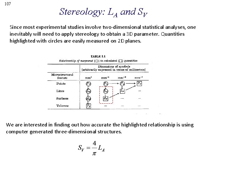
14 Measured vs. Derived Quantities Remember that it is very difficult to obtain true 3 D measurements (squares) and so we must find stereological methods to estimate the 3 D quantities (squares) from 2 D measurements (circles). Objectives Notation Equations Delesse SV-PL LA-PL Topology Grain_Size Distributions

15 Volume Fraction • Typical method of measurement is to identify phases by contrast (gray level, color) and either use pixel counting (point counting) or line intercepts. • Volume fractions, surface area (per unit volume), diameters and curvatures are readily obtained. Objectives Notation Equations Delesse SV-PL LA-PL Topology Grain_Size Distributions

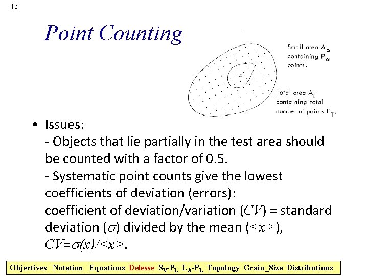
16 Point Counting • Issues: - Objects that lie partially in the test area should be counted with a factor of 0. 5. - Systematic point counts give the lowest coefficients of deviation (errors): coefficient of deviation/variation (CV) = standard deviation (s) divided by the mean (<x>), CV=s(x)/<x>. Objectives Notation Equations Delesse SV-PL LA-PL Topology Grain_Size Distributions

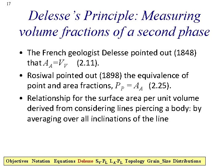
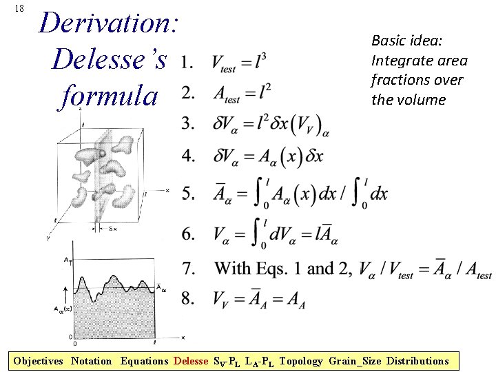
17 Delesse’s Principle: Measuring volume fractions of a second phase • The French geologist Delesse pointed out (1848) that AA=VV (2. 11). • Rosiwal pointed out (1898) the equivalence of point and area fractions, PP = AA (2. 25). • Relationship for the surface area per unit volume derived from considering lines piercing a body: by averaging over all inclinations of the line Objectives Notation Equations Delesse SV-PL LA-PL Topology Grain_Size Distributions

18 Derivation: Delesse’s formula Basic idea: Integrate area fractions over the volume Objectives Notation Equations Delesse SV-PL LA-PL Topology Grain_Size Distributions

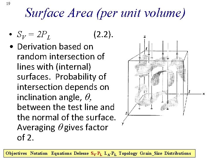
19 Surface Area (per unit volume) • SV = 2 PL (2. 2). • Derivation based on random intersection of lines with (internal) surfaces. Probability of intersection depends on inclination angle, between the test line and the normal of the surface. Averaging gives factor of 2. Objectives Notation Equations Delesse SV-PL LA-PL Topology Grain_Size Distributions

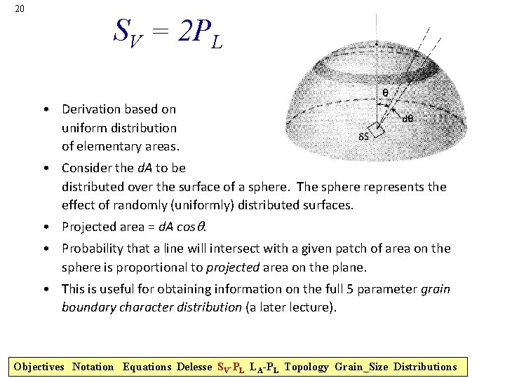
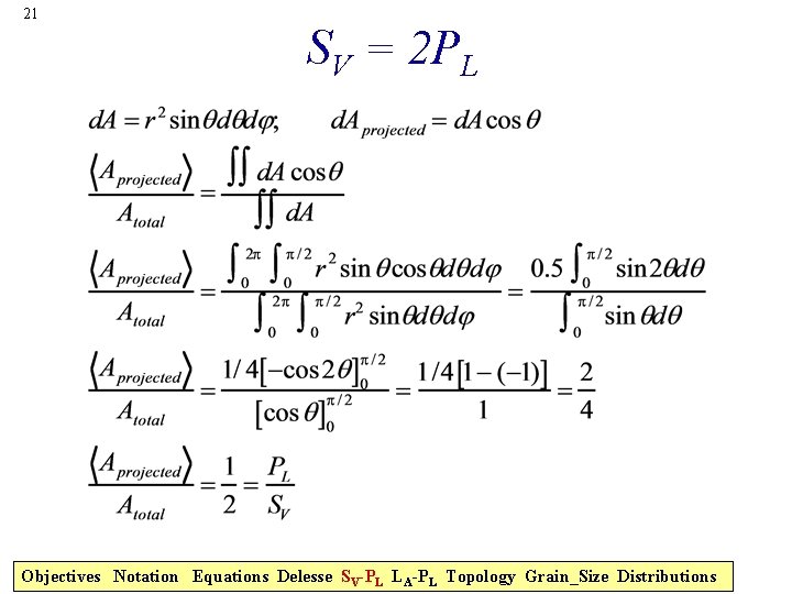
20 SV = 2 PL • Derivation based on uniform distribution of elementary areas. • Consider the d. A to be distributed over the surface of a sphere. The sphere represents the effect of randomly (uniformly) distributed surfaces. • Projected area = d. A cos. • Probability that a line will intersect with a given patch of area on the sphere is proportional to projected area on the plane. • This is useful for obtaining information on the full 5 parameter grain boundary character distribution (a later lecture). Objectives Notation Equations Delesse SV-PL LA-PL Topology Grain_Size Distributions

21 SV = 2 PL Objectives Notation Equations Delesse SV-PL LA-PL Topology Grain_Size Distributions

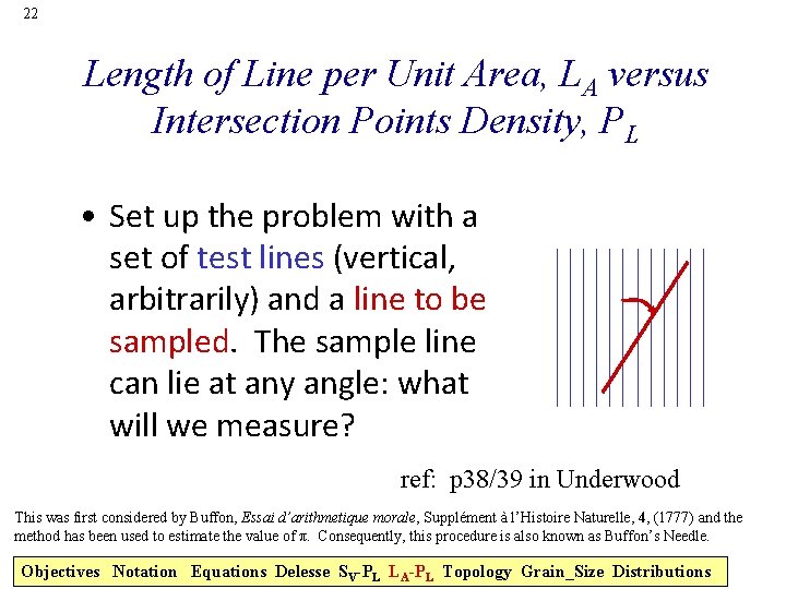
22 Length of Line per Unit Area, LA versus Intersection Points Density, PL • Set up the problem with a set of test lines (vertical, arbitrarily) and a line to be sampled. The sample line can lie at any angle: what will we measure? ref: p 38/39 in Underwood This was first considered by Buffon, Essai d’arithmetique morale, Supplément à l’Histoire Naturelle, 4, (1777) and the method has been used to estimate the value of π. Consequently, this procedure is also known as Buffon’s Needle. Objectives Notation Equations Delesse SV-PL LA-PL Topology Grain_Size Distributions

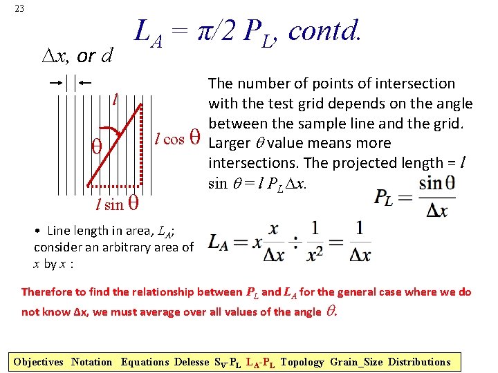
23 ∆x, or d LA = π/2 PL, contd. l q l cos q l sin q The number of points of intersection with the test grid depends on the angle between the sample line and the grid. Larger value means more intersections. The projected length = l sin = l PL ∆x. • Line length in area, LA; consider an arbitrary area of x by x : Therefore to find the relationship between PL and LA for the general case where we do not know ∆x, we must average over all values of the angle Objectives Notation Equations Delesse SV-PL LA-PL Topology Grain_Size Distributions

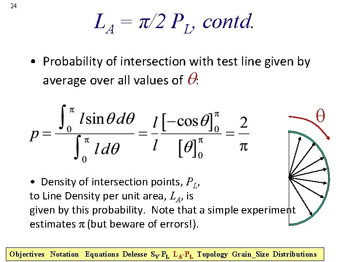
24 LA = π/2 PL, contd. • Probability of intersection with test line given by average over all values of : q • Density of intersection points, PL, to Line Density per unit area, LA, is given by this probability. Note that a simple experiment estimates π (but beware of errors!). Objectives Notation Equations Delesse SV-PL LA-PL Topology Grain_Size Distributions

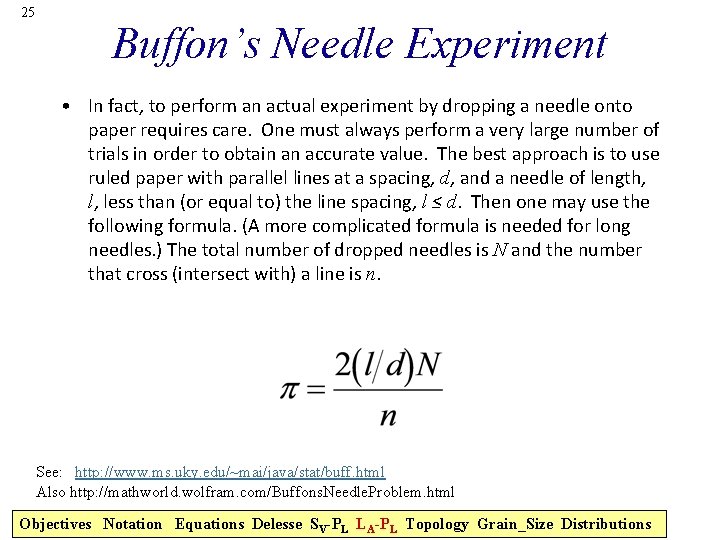
25 Buffon’s Needle Experiment • In fact, to perform an actual experiment by dropping a needle onto paper requires care. One must always perform a very large number of trials in order to obtain an accurate value. The best approach is to use ruled paper with parallel lines at a spacing, d, and a needle of length, l, less than (or equal to) the line spacing, l ≤ d. Then one may use the following formula. (A more complicated formula is needed for long needles. ) The total number of dropped needles is N and the number that cross (intersect with) a line is n. See: http: //www. ms. uky. edu/~mai/java/stat/buff. html Also http: //mathworld. wolfram. com/Buffons. Needle. Problem. html Objectives Notation Equations Delesse SV-PL LA-PL Topology Grain_Size Distributions

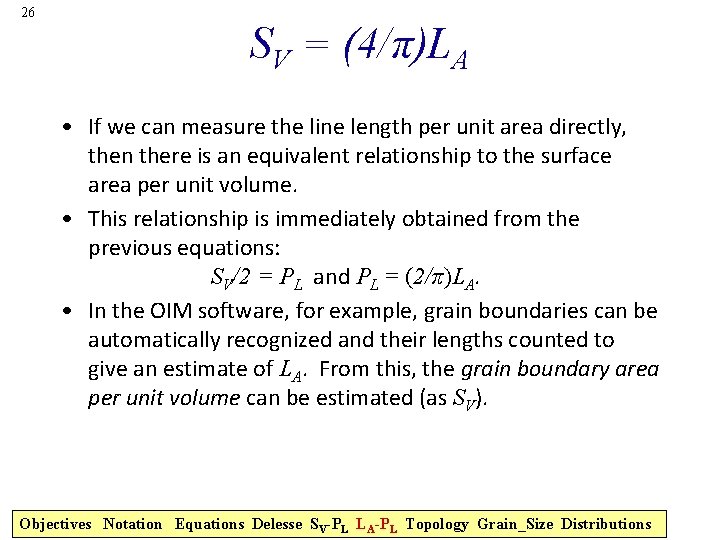
26 SV = (4/π)LA • If we can measure the line length per unit area directly, then there is an equivalent relationship to the surface area per unit volume. • This relationship is immediately obtained from the previous equations: SV/2 = PL and PL = (2/π)LA. • In the OIM software, for example, grain boundaries can be automatically recognized and their lengths counted to give an estimate of LA. From this, the grain boundary area per unit volume can be estimated (as SV). Objectives Notation Equations Delesse SV-PL LA-PL Topology Grain_Size Distributions

27 Outline • Objectives • Motivation • Quantities, – definitions – measurable – Derivable • Problems that use Stereology, Topology • Volume fractions • Surface area per unit volume • Facet areas • Oriented objects • Particle spacings – Mean Free Path – Nearest Neighbor Distance • Zener Pinning • Grain Size • Sections through objects – Size Distributions

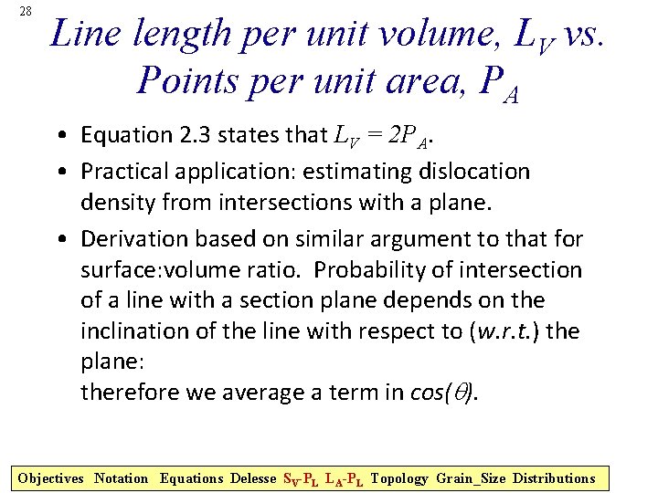
28 Line length per unit volume, LV vs. Points per unit area, PA • Equation 2. 3 states that LV = 2 PA. • Practical application: estimating dislocation density from intersections with a plane. • Derivation based on similar argument to that for surface: volume ratio. Probability of intersection of a line with a section plane depends on the inclination of the line with respect to (w. r. t. ) the plane: therefore we average a term in cos( ). Objectives Notation Equations Delesse SV-PL LA-PL Topology Grain_Size Distributions

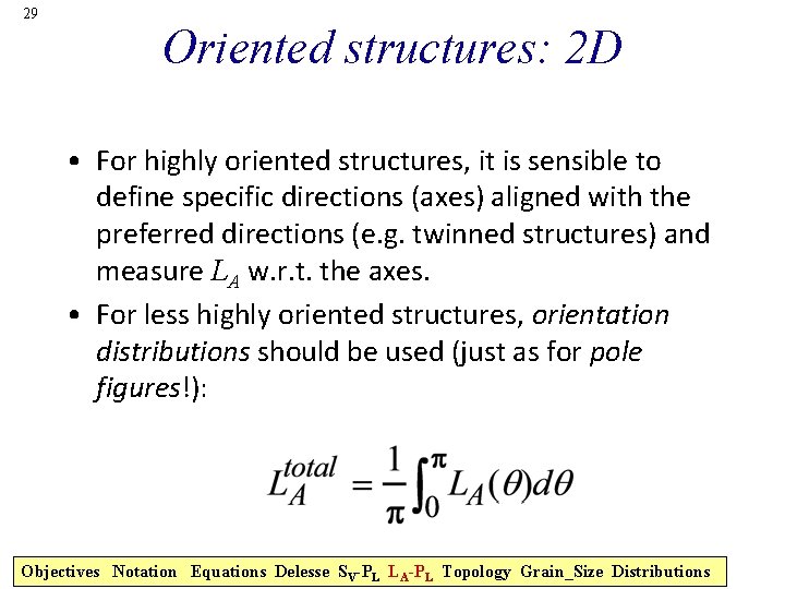
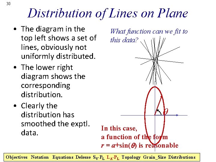
29 Oriented structures: 2 D • For highly oriented structures, it is sensible to define specific directions (axes) aligned with the preferred directions (e. g. twinned structures) and measure LA w. r. t. the axes. • For less highly oriented structures, orientation distributions should be used (just as for pole figures!): Objectives Notation Equations Delesse SV-PL LA-PL Topology Grain_Size Distributions

30 Distribution of Lines on Plane • The diagram in the What function can we fit to top left shows a set of this data? lines, obviously not uniformly distributed. • The lower right diagram shows the corresponding distribution. • Clearly the distribution has smoothed the exptl. In this case, data. a function of the form r = a+sin(q) is reasonable Objectives Notation Equations Delesse SV-PL LA-PL Topology Grain_Size Distributions

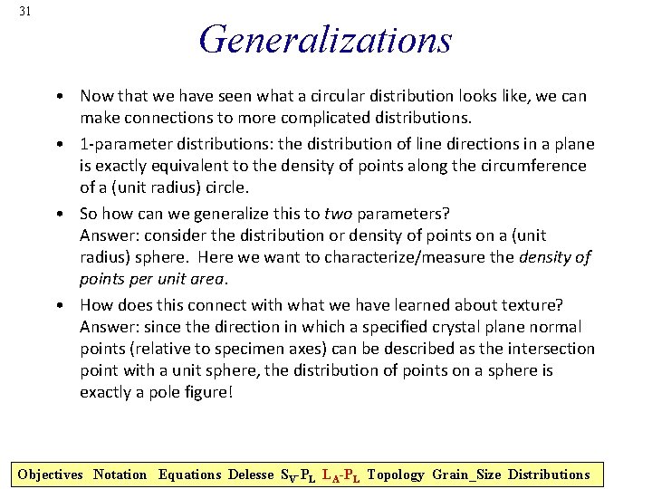
31 Generalizations • Now that we have seen what a circular distribution looks like, we can make connections to more complicated distributions. • 1 -parameter distributions: the distribution of line directions in a plane is exactly equivalent to the density of points along the circumference of a (unit radius) circle. • So how can we generalize this to two parameters? Answer: consider the distribution or density of points on a (unit radius) sphere. Here we want to characterize/measure the density of points per unit area. • How does this connect with what we have learned about texture? Answer: since the direction in which a specified crystal plane normal points (relative to specimen axes) can be described as the intersection point with a unit sphere, the distribution of points on a sphere is exactly a pole figure! Objectives Notation Equations Delesse SV-PL LA-PL Topology Grain_Size Distributions

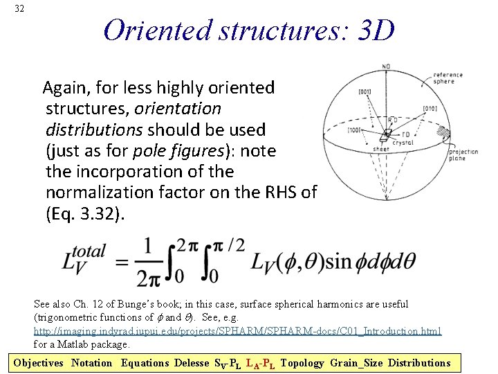
32 Oriented structures: 3 D Again, for less highly oriented structures, orientation distributions should be used (just as for pole figures): note the incorporation of the normalization factor on the RHS of (Eq. 3. 32). See also Ch. 12 of Bunge’s book; in this case, surface spherical harmonics are useful (trigonometric functions of f and ). See, e. g. http: //imaging. indyrad. iupui. edu/projects/SPHARM-docs/C 01_Introduction. html for a Matlab package. Objectives Notation Equations Delesse SV-PL LA-PL Topology Grain_Size Distributions

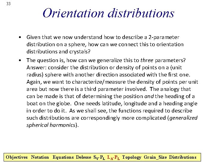
33 Orientation distributions • Given that we now understand how to describe a 2 -parameter distribution on a sphere, how can we connect this to orientation distributions and crystals? • The question is, how can we generalize this to three parameters? Answer: consider the distribution or density of points on a (unit radius) sphere with another direction associated with the first one. Again, we want to characterize/measure the density of points per unit area but now there is a third parameter involved. The analogy that can be made is that of determining the position and the heading of a boat on the globe. One needs latitude, longitude and a heading angle in order to do it. As we shall see, the functions required to describe such distributions are correspondingly more complicated (generalized spherical harmonics). Objectives Notation Equations Delesse SV-PL LA-PL Topology Grain_Size Distributions

34 Outline • Objectives • Motivation • Quantities, – definitions – measurable – Derivable • Problems that use Stereology, Topology • Volume fractions • Surface area per unit volume • Facet areas • Oriented objects • Particle spacings – Mean Free Path – Nearest Neighbor Distance • Zener Pinning • Grain Size • Sections through objects – Size Distributions

35 Second Phase Particles • Now we consider second phase particles • Although the derivations are general, we mostly deal with small volume fractions of convex, (nearly) spherical particles • Quantities of interest: – intercept length, PL or NL – particle spacing, ∆ – mean free path, (or uninterrupted distance between particles)

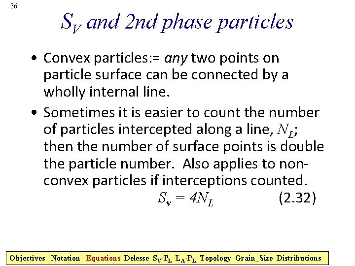
36 SV and 2 nd phase particles • Convex particles: = any two points on particle surface can be connected by a wholly internal line. • Sometimes it is easier to count the number of particles intercepted along a line, NL; then the number of surface points is double the particle number. Also applies to nonconvex particles if interceptions counted. Sv = 4 NL (2. 32) Objectives Notation Equations Delesse SV-PL LA-PL Topology Grain_Size Distributions

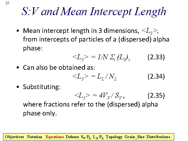
37 S: V and Mean Intercept Length • Mean intercept length in 3 dimensions, <L 3>, from intercepts of particles of a (dispersed) alpha phase: <L 3> = 1/N Si (L 3)i (2. 33) • Can also be obtained as: <L 3> = LL / NL (2. 34) • Substituting: <L 3> = 4 VV / SV , (2. 35) where fractions refer to the (dispersed) alpha phase only. Objectives Notation Equations Delesse SV-PL LA-PL Topology Grain_Size Distributions

38 S: V example: sphere • For a sphere, the volume: surface ratio (=VV/SV) is D[iameter]/6. • Thus <L 3>sphere = 2 D/3. • In general we can invert the relationship to obtain the surface: volume ratio, if we know (or measure) the mean intercept: <S/V>alpha = 4/<L 3> (2. 38) Objectives Notation Equations Delesse SV-PL LA-PL Topology Grain_Size Distributions

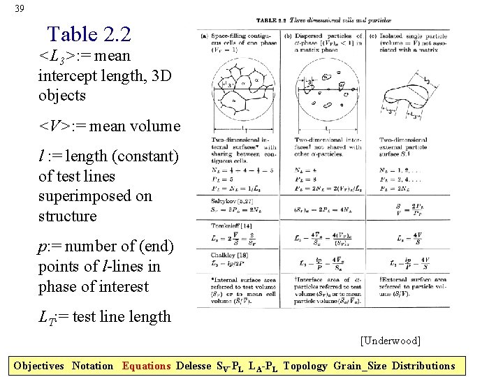
39 Table 2. 2 <L 3>: = mean intercept length, 3 D objects <V>: = mean volume l : = length (constant) of test lines superimposed on structure p: = number of (end) points of l-lines in phase of interest LT: = test line length [Underwood] Objectives Notation Equations Delesse SV-PL LA-PL Topology Grain_Size Distributions

40 Grain size measurement: intercepts • From Table 2. 2 [Underwood], column (a), illustrates how to make a measurement of the mean intercept length, based on the number of grains per unit length of test line. <L 3> = 1/NL • Important: use many test lines that are randomly oriented w. r. t. the structure. • Assuming spherical† grains, <L 3> = 4 r/3, [Underwood, Table 4. 1], there are 5 intersections and if we take the total test line length, LT= 25µm, then LTNL= 5, so NL= 1/5 µm-1 d = 2 r = 6<L 3>/4 = 6/NL 4 = 6*5/4 = 7. 5µm. † Ask yourself what a better assumption about grain shape might be! Objectives Notation Equations Delesse SV-PL LA-PL Topology Grain_Size Distributions

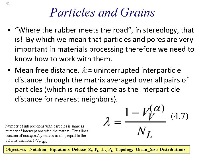
41 Particles and Grains • “Where the rubber meets the road”, in stereology, that is! By which we mean that particles and pores are very important in materials processing therefore we need to know how to work with them. • Mean free distance, : = uninterrupted interparticle distance through the matrix averaged over all pairs of particles (which is not the same as the interparticle distance for nearest neighbors). (4. 7) Number of interceptions with particles is same as number of interceptions with the matrix. Thus lineal fraction of occupied by matrix is NL, equal to the volume fraction, 1 -VV-alpha. Objectives Notation Equations Delesse SV-PL LA-PL Topology Grain_Size Distributions

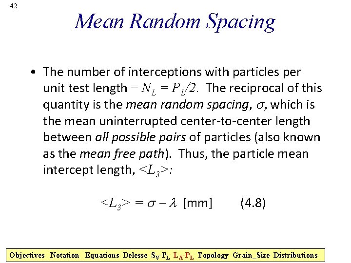
42 Mean Random Spacing • The number of interceptions with particles per unit test length = NL = PL/2. The reciprocal of this quantity is the mean random spacing, s which is the mean uninterrupted center-to-center length between all possible pairs of particles (also known as the mean free path). Thus, the particle mean intercept length, <L 3>: <L 3> = s - [mm] (4. 8) Objectives Notation Equations Delesse SV-PL LA-PL Topology Grain_Size Distributions

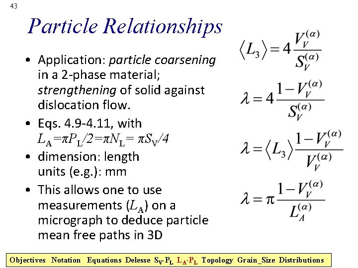
43 Particle Relationships • Application: particle coarsening in a 2 -phase material; strengthening of solid against dislocation flow. • Eqs. 4. 9 -4. 11, with LA=πPL/2=πNL= πSV/4 • dimension: length units (e. g. ): mm • This allows one to use measurements (LA) on a micrograph to deduce particle mean free paths in 3 D Objectives Notation Equations Delesse SV-PL LA-PL Topology Grain_Size Distributions

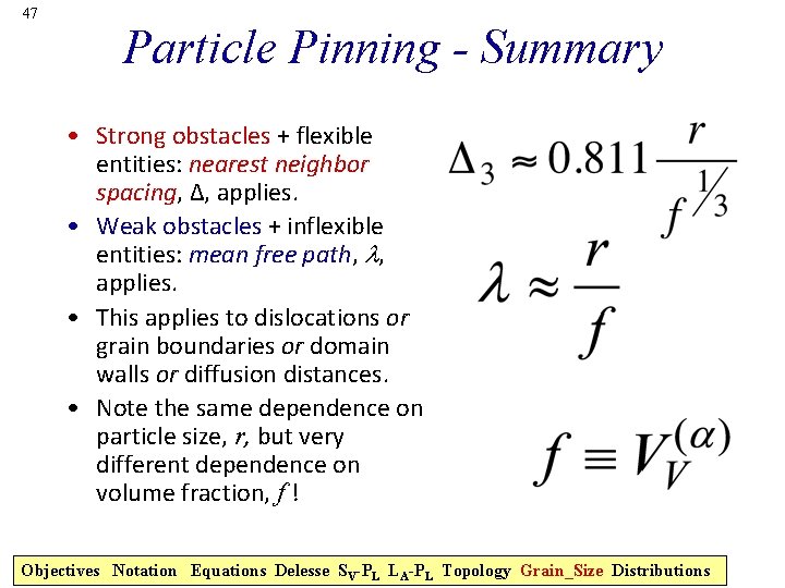
44 Mean free path, , versus Nearest neighbor spacing, ∆ • It is useful (and therefore important) to keep the difference between mean free path and nearest neighbor spacing separate and distinct. • Mean free path is how far, on average, you travel from one particle until you encounter another one. • Nearest neighbor spacing is how far apart, on average, two nearest neighbors are from each other. Matters for diffusion distances, e. g. • They appear at first glance to be the same thing but they are not! • They are related to one another, as we shall see in the next few slides. • This matters, e. g. , when considering dislocations moving past obstacles, which may be effectively rigid lines (weak obstacles) or flexible (strong obstacles). Objectives Notation Equations Delesse SV-PL LA-PL Topology Grain_Size Distributions

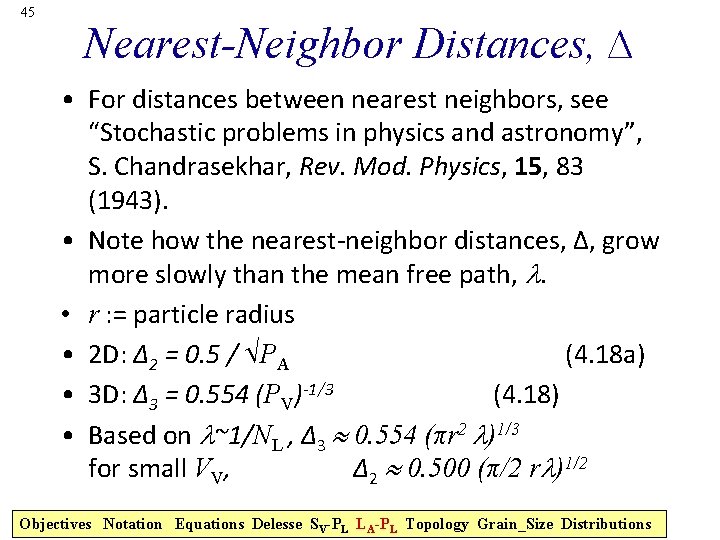
45 Nearest-Neighbor Distances, ∆ • For distances between nearest neighbors, see “Stochastic problems in physics and astronomy”, S. Chandrasekhar, Rev. Mod. Physics, 15, 83 (1943). • Note how the nearest-neighbor distances, ∆, grow more slowly than the mean free path, . • r : = particle radius • 2 D: ∆2 = 0. 5 / √PA (4. 18 a) • 3 D: ∆3 = 0. 554 (PV)-1/3 (4. 18) • Based on ~1/NL , ∆3 0. 554 (πr 2 )1/3 for small VV, ∆2 0. 500 (π/2 r )1/2 Objectives Notation Equations Delesse SV-PL LA-PL Topology Grain_Size Distributions

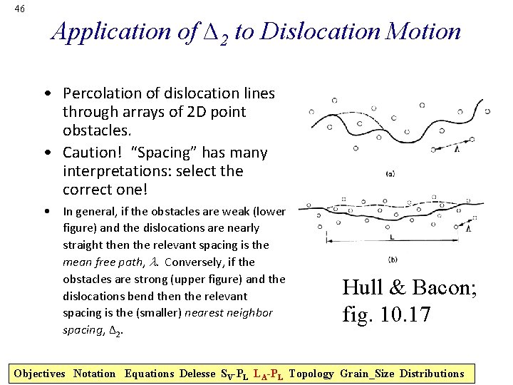
46 Application of ∆2 to Dislocation Motion • Percolation of dislocation lines through arrays of 2 D point obstacles. • Caution! “Spacing” has many interpretations: select the correct one! • In general, if the obstacles are weak (lower figure) and the dislocations are nearly straight then the relevant spacing is the mean free path, . Conversely, if the obstacles are strong (upper figure) and the dislocations bend then the relevant spacing is the (smaller) nearest neighbor spacing, ∆2. Hull & Bacon; fig. 10. 17 Objectives Notation Equations Delesse SV-PL LA-PL Topology Grain_Size Distributions

47 Particle Pinning - Summary • Strong obstacles + flexible entities: nearest neighbor spacing, ∆, applies. • Weak obstacles + inflexible entities: mean free path, , applies. • This applies to dislocations or grain boundaries or domain walls or diffusion distances. • Note the same dependence on particle size, r, but very different dependence on volume fraction, f ! Objectives Notation Equations Delesse SV-PL LA-PL Topology Grain_Size Distributions

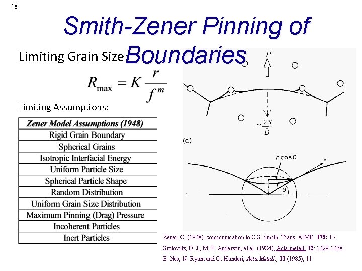
48 Smith-Zener Pinning of Limiting Grain Size: Boundaries Limiting Assumptions: Zener, C. (1948). communication to C. S. Smith. Trans. AIME. 175: 15. Srolovitz, D. J. , M. P. Anderson, et al. (1984), Acta metall. 32: 1429 -1438. E. Nes, N. Ryum and O. Hunderi, Acta Metall. , 33 (1985), 11

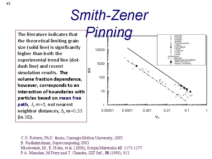
49 Smith-Zener Pinning The literature indicates that theoretical limiting grain size (solid line) is significantly higher than both the experimental trend line (dotdash line) and recent simulation results. The volume fraction dependence, however, corresponds to an interaction of boundaries with particles based on mean free path, , m=1, not nearest neighbor distances, ∆, m=0. 33 (in 3 D). C. G. Roberts, Ph. D. thesis, Carnegie Mellon University, 2007. B. Radhakrishnan, Supercomputing 2003. Miodownik, M. , E. Holm, et al. (2000), Scripta Materialia 42: 1173 -1177. P. A. Manohar, M. Ferry and T. Chandra, ISIJ Intl. , 38 (1998), 913.

50 From discussion with C. Roberts, 16 Aug 06 Particles on boundaries, in cross-section An interesting question is to compare the number of particles on boundaries, as a fraction of the total particles in view in a crosssection. We can use the analysis provided by Underwood to arrive at an estimate. If, for example, boundaries have pinned out during grain growth, one might expect the measured fraction on boundaries to be higher than this estimate based on random intersection. - (NA)b is the number of particles per unit area in contact with boundaries. - LA is the line length per unit area of (grain) boundary. - The other quantities have their usual meanings. See: "Particle-Associated Misorientation Distribution in a Nickel-Base Superalloy". Roberts C. G. , Semiatin S. L. , Rollett A. D. , Scripta materialia 56 899 -902 (2007).

51 Outline • Objectives • Motivation • Quantities, – definitions – measurable – Derivable • Problems that use Stereology, Topology • Volume fractions • Surface area per unit volume • Facet areas • Oriented objects • Particle spacings – Mean Free Path – Nearest Neighbor Distance • Zener Pinning • Grain Size • Sections through objects – Size Distributions

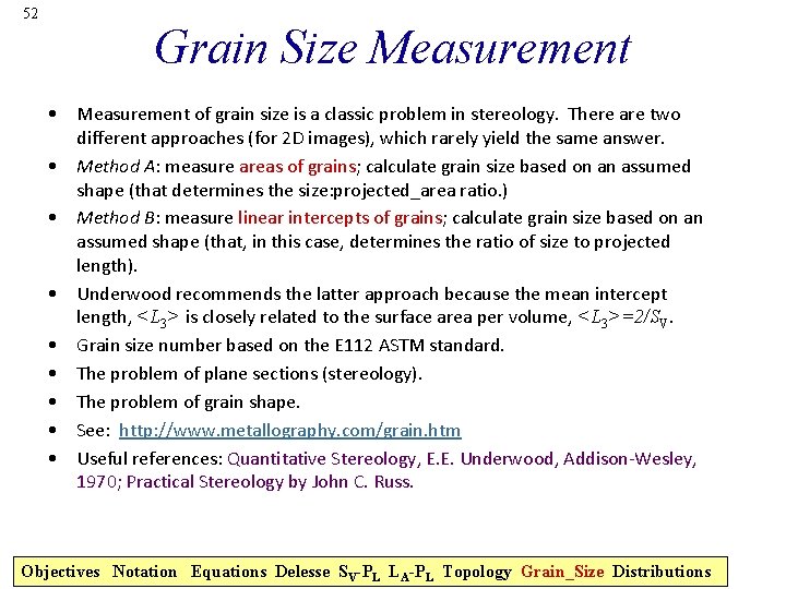
52 Grain Size Measurement • Measurement of grain size is a classic problem in stereology. There are two different approaches (for 2 D images), which rarely yield the same answer. • Method A: measure areas of grains; calculate grain size based on an assumed shape (that determines the size: projected_area ratio. ) • Method B: measure linear intercepts of grains; calculate grain size based on an assumed shape (that, in this case, determines the ratio of size to projected length). • Underwood recommends the latter approach because the mean intercept length, <L 3> is closely related to the surface area per volume, <L 3>=2/SV. • Grain size number based on the E 112 ASTM standard. • The problem of plane sections (stereology). • The problem of grain shape. • See: http: //www. metallography. com/grain. htm • Useful references: Quantitative Stereology, E. E. Underwood, Addison-Wesley, 1970; Practical Stereology by John C. Russ. Objectives Notation Equations Delesse SV-PL LA-PL Topology Grain_Size Distributions

53 Method A: typical section [Underwood] • Correction terms (Eb, C 1’, C 2’) allow finite sections to be interpreted. C 1’: =number of incomplete corners against 1 polygon; C 2’: = same for 2 polygons Objectives Notation Equations Delesse SV-PL LA-PL Topology Grain_Size Distributions

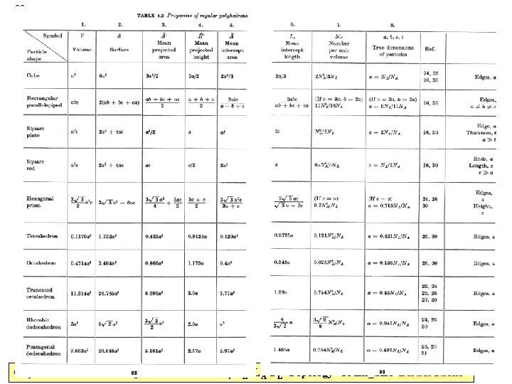
54 Method A: area based [Underwood] Fig. 7. 12 • Grain count method: <A>=1/NA • Number of whole grains= 20 Number of edge grains= 21 Effective total = Nwhole+Nedge/2 = 30. 5 Total area= 0. 5 mm 2 Thus, NA= 61 mm-2; <A>=16, 400 µm 2 • Assume spherical* grains, <A> mean intercept area= 2/3πr 2 d = 2√(3<A>/2π)= 177 µm. *Do you think this is a reasonable assumption? ! [Underwood] Objectives Notation Equations Delesse SV-PL LA-PL Topology Grain_Size Distributions

55 Method B: linear intercept • From Table 2. 2 [Underwood], column (a), illustrates how to make a measurement of the mean intercept length, based on the number of grains per unit length of test line. <L 3> = 1/NL • Important: use many test lines that are randomly oriented w. r. t. the structure. • Assuming spherical† grains, <L 3> = 4 r/3, [Underwood, Table 4. 1], if we take the total line length (diameter of test area), LT= 798µm, and draw a line that intersects 7 boundaries, then NL= 1/114 µm-1 d = 6<L 3>/4 = 6/NL 4 = 6*114/4 = 171 µm. • Clearly the two measures of grain size are similar but not necessarily the same. † Ask yourself what a better assumption about grain shape might be! Objectives Notation Equations Delesse SV-PL LA-PL Topology Grain_Size Distributions

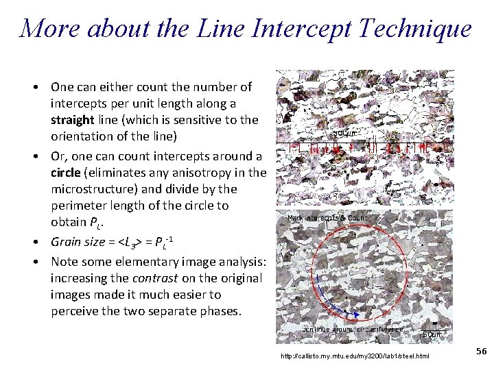
More about the Line Intercept Technique • One can either count the number of intercepts per unit length along a straight line (which is sensitive to the orientation of the line) • Or, one can count intercepts around a circle (eliminates any anisotropy in the microstructure) and divide by the perimeter length of the circle to obtain PL. • Grain size = <L 3> = PL-1 • Note some elementary image analysis: increasing the contrast on the original images made it much easier to perceive the two separate phases. http: //callisto. my. mtu. edu/my 3200/lab 1/steel. html 56

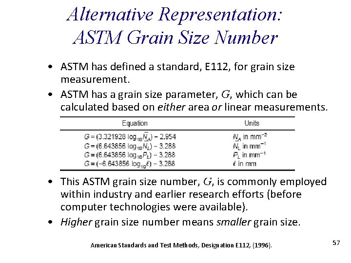
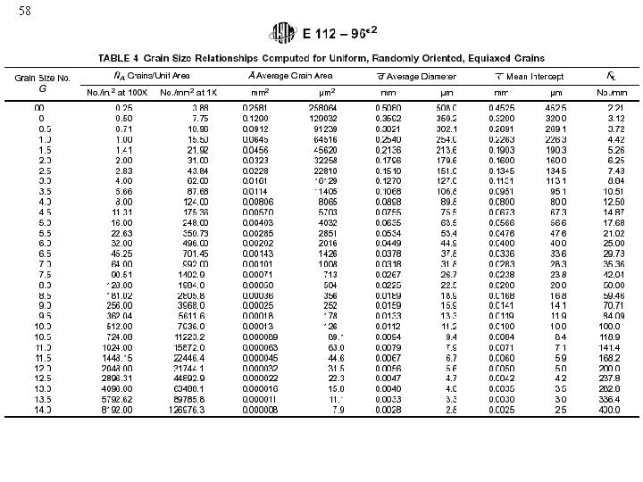
Alternative Representation: ASTM Grain Size Number • ASTM has defined a standard, E 112, for grain size measurement. • ASTM has a grain size parameter, G, which can be calculated based on either area or linear measurements. • This ASTM grain size number, G, is commonly employed within industry and earlier research efforts (before computer technologies were available). • Higher grain size number means smaller grain size. American Standards and Test Methods, Designation E 112, (1996). 57

58

59 Outline • Objectives • Motivation • Quantities, – definitions – measurable – Derivable • Problems that use Stereology, Topology • Volume fractions • Surface area per unit volume • Facet areas • Oriented objects • Particle spacings – Mean Free Path – Nearest Neighbor Distance • Zener Pinning • Grain Size • Sections through objects – Size Distributions

60 3 D Size Derived from 2 D Sections • Purpose: how can we relate measurements in plane sections to what we know of the geometry of regularly shaped objects with a distribution of sizes? • In general, the mean intercept length is not equal to the grain diameter, for example! Also, the proportionality factors depend on the (assumed) shape. • Example: for monodisperse spherical particles (all the same size) distributed (randomly) in space, sectioning through them and measuring the size distribution will show a spread in apparent size. Objectives Notation Equations Delesse SV-PL LA-PL Topology Grain_Size Distributions

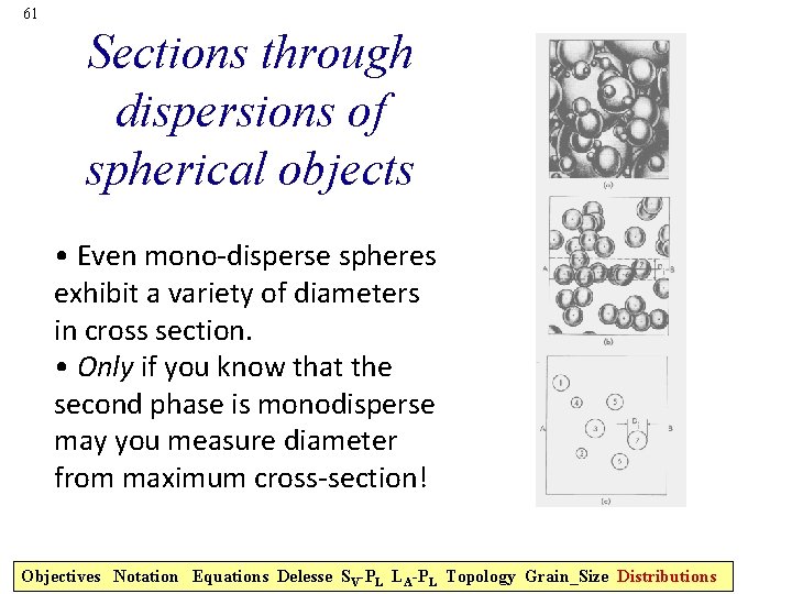
61 Sections through dispersions of spherical objects • Even mono-disperse spheres exhibit a variety of diameters in cross section. • Only if you know that the second phase is monodisperse may you measure diameter from maximum cross-section! Objectives Notation Equations Delesse SV-PL LA-PL Topology Grain_Size Distributions

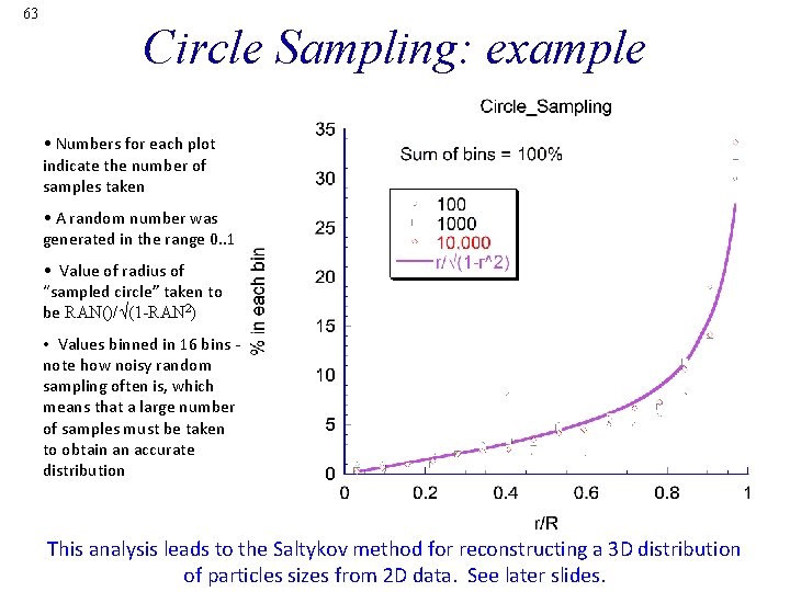
62 [Russ & De. Hoff, Ch. 12] Sectioning Spheres • The radius, r, of a circle sectioned at a distance h from the center is r = √(R 2 -h 2). • Since the sectioning planes intersect a sphere at a random location relative to its size, R, we can assume that the probability of observing a circle between a given intercept radius, r, and r+dr, is equal to the relative thickness, dz/R, of the corresponding slice. • The result is a distribution of intercept sizes that varies between zero and the actual sphere size.

63 Circle Sampling: example • Numbers for each plot indicate the number of samples taken • A random number was generated in the range 0. . 1 • Value of radius of “sampled circle” taken to be RAN()/√(1 -RAN 2) • Values binned in 16 bins - note how noisy random sampling often is, which means that a large number of samples must be taken to obtain an accurate distribution This analysis leads to the Saltykov method for reconstructing a 3 D distribution of particles sizes from 2 D data. See later slides.

64 Distributions of Sizes • Measurement of an average quantity is reasonably straightforward in stereology. • Deduction of a 3 D size distribution from the projection of that distribution on a section plane is much less straightforward (and still controversial in certain respects). • Example: it is useful to be able to measure particle size and grain size distributions from plane sections (without resorting to serial sectioning). • Assumptions about particle shape must be made. Objectives Notation Equations Delesse SV-PL LA-PL Topology Grain_Size Distributions

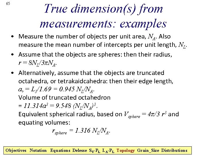
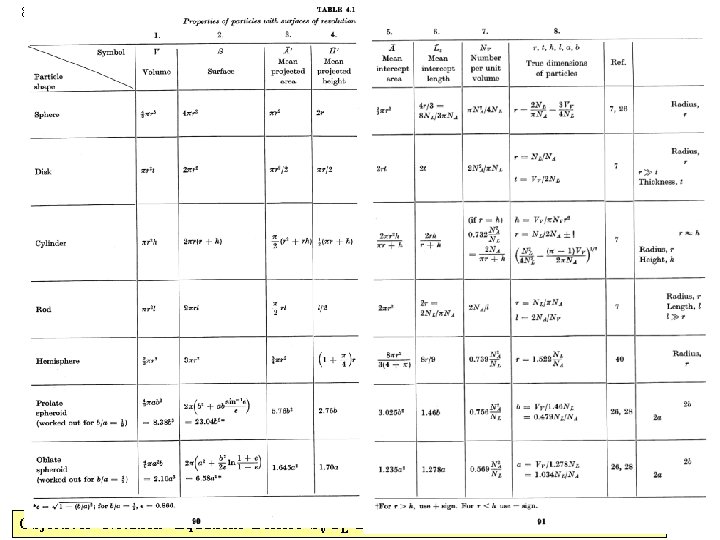
65 True dimension(s) from measurements: examples • Measure the number of objects per unit area, NA. Also measure the mean number of intercepts per unit length, NL. • Assume that the objects are spheres: then their radius, r = 8 NL/3πNA. • Alternatively, assume that the objects are truncated octahedra, or tetrakaidcahedra: then their edge length, a, = L 3/1. 69 = 0. 945 NL/NA. Volume of truncated octahedron = 11. 314 a 3 = 9. 548 (NL/NA)3. Equivalent spherical radius, based on Vsphere = 4π/3 r 3 and equating volumes: rsphere = 1. 316 NL/NA. Objectives Notation Equations Delesse SV-PL LA-PL Topology Grain_Size Distributions

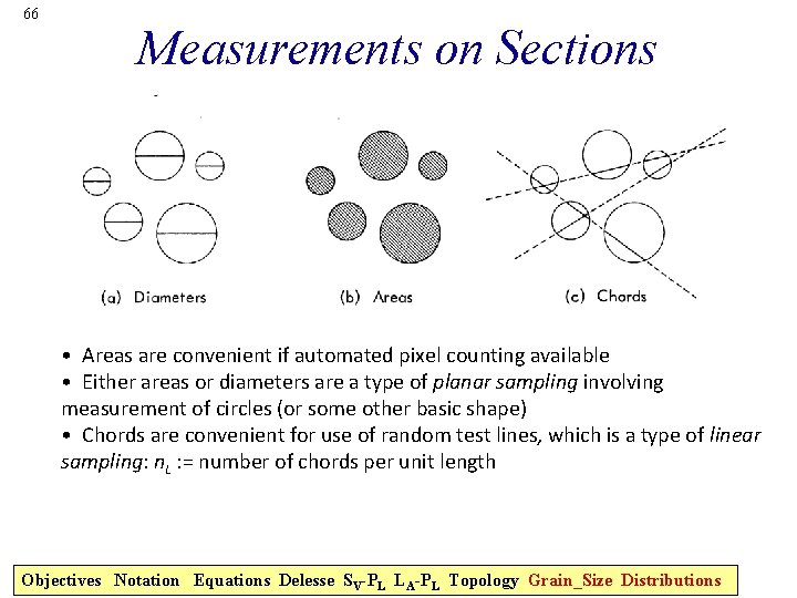
66 Measurements on Sections • Areas are convenient if automated pixel counting available • Either areas or diameters are a type of planar sampling involving measurement of circles (or some other basic shape) • Chords are convenient for use of random test lines, which is a type of linear sampling: n. L : = number of chords per unit length Objectives Notation Equations Delesse SV-PL LA-PL Topology Grain_Size Distributions

67 Extraction of Size Distribution • Whenever you section a distribution of particles of a finite size, the section plane is unlikely to cut at the maximum diameter (of, say, spherical particles). • Therefore the observed sizes are always an underestimate of the actual sizes. • Any method for estimating size distributions in effect starts with the largest size class and, based on some assumption about the shape and distribution of the particles, reduces the volume fraction of the next smallest size class by an amount that is proportional to the fraction of the current size class.

68 Size distributions from measurement • Distribution of cross sections very different from 3 D size distribution, as illustrated with monosize spheres. • Measurement of chord lengths is most reliable, i. e. experimental frequency of n. L(l) versus l. • See articles by Lord & Willis; Cahn & Fullman; book by Saltykov • <D> : = mean diameter; s(D): = standard deviation NV : = number of particles (grains) per unit volume. Objectives Notation Equations Delesse SV-PL LA-PL Topology Grain_Size Distributions

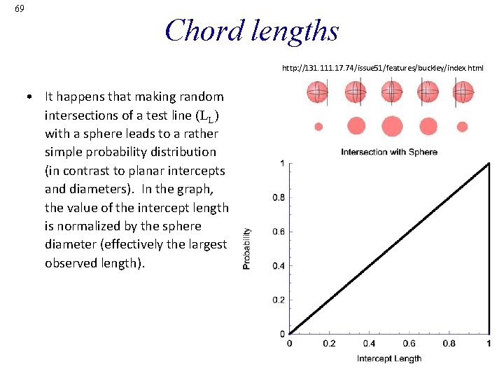
69 Chord lengths http: //131. 111. 17. 74/issue 51/features/buckley/index. html • It happens that making random intersections of a test line (LL) with a sphere leads to a rather simple probability distribution (in contrast to planar intercepts and diameters). In the graph, the value of the intercept length is normalized by the sphere diameter (effectively the largest observed length).

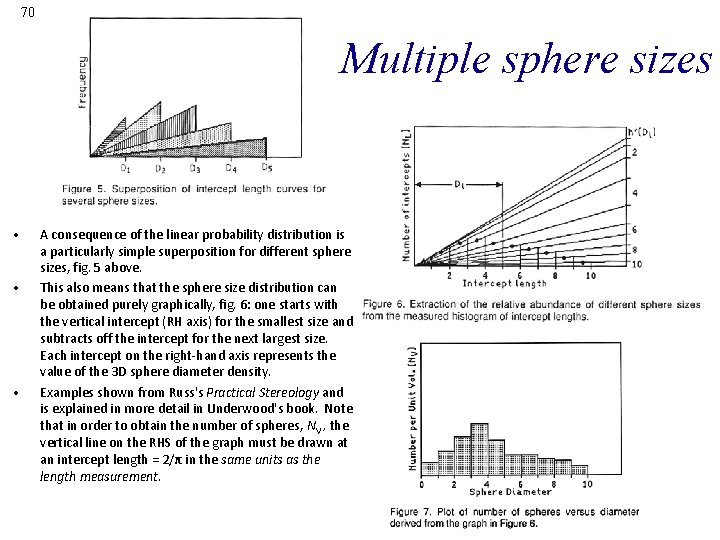
70 Multiple sphere sizes • • • A consequence of the linear probability distribution is a particularly simple superposition for different sphere sizes, fig. 5 above. This also means that the sphere size distribution can be obtained purely graphically, fig. 6: one starts with the vertical intercept (RH axis) for the smallest size and subtracts off the intercept for the next largest size. Each intercept on the right-hand axis represents the value of the 3 D sphere diameter density. Examples shown from Russ's Practical Stereology and is explained in more detail in Underwood's book. Note that in order to obtain the number of spheres, NV , the vertical line on the RHS of the graph must be drawn at an intercept length = 2/π in the same units as the length measurement.

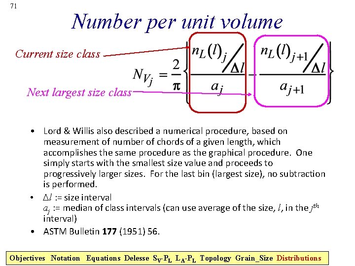
71 Number per unit volume Current size class Next largest size class • Lord & Willis also described a numerical procedure, based on measurement of number of chords of a given length, which accomplishes the same procedure as the graphical procedure. One simply starts with the smallest size value and proceeds to progressively larger sizes. For the last bin (largest size), no subtraction is performed. • ∆l : = size interval aj : = median of class intervals (can use average of the size, l, in the jth interval) • ASTM Bulletin 177 (1951) 56. Objectives Notation Equations Delesse SV-PL LA-PL Topology Grain_Size Distributions

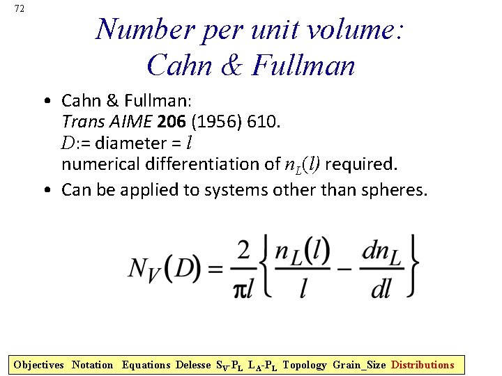
72 Number per unit volume: Cahn & Fullman • Cahn & Fullman: Trans AIME 206 (1956) 610. D: = diameter = l numerical differentiation of n. L(l) required. • Can be applied to systems other than spheres. Objectives Notation Equations Delesse SV-PL LA-PL Topology Grain_Size Distributions

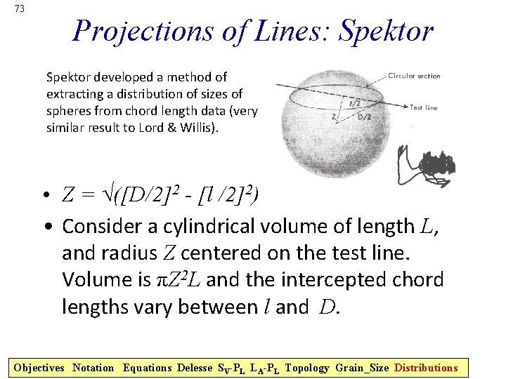
73 Projections of Lines: Spektor developed a method of extracting a distribution of sizes of spheres from chord length data (very similar result to Lord & Willis). • Z = √([D/2]2 - [l /2]2) • Consider a cylindrical volume of length L, and radius Z centered on the test line. Volume is πZ 2 L and the intercepted chord lengths vary between l and D. Objectives Notation Equations Delesse SV-PL LA-PL Topology Grain_Size Distributions

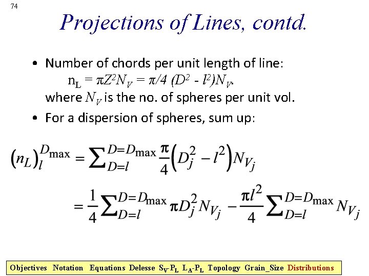
74 Projections of Lines, contd. • Number of chords per unit length of line: n. L = πZ 2 NV = π/4 (D 2 - l 2)NV. where NV is the no. of spheres per unit vol. • For a dispersion of spheres, sum up: Objectives Notation Equations Delesse SV-PL LA-PL Topology Grain_Size Distributions

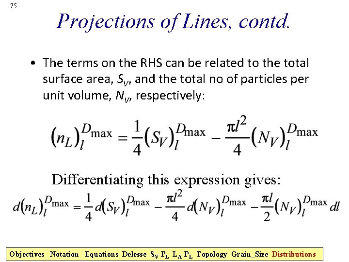
75 Projections of Lines, contd. • The terms on the RHS can be related to the total surface area, SV, and the total no of particles per unit volume, NV, respectively: Differentiating this expression gives: Objectives Notation Equations Delesse SV-PL LA-PL Topology Grain_Size Distributions

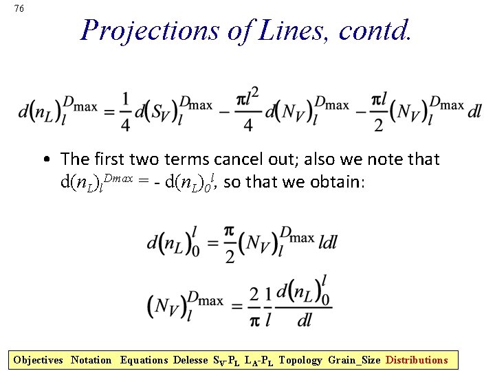
76 Projections of Lines, contd. • The first two terms cancel out; also we note that d(n. L)l. Dmax = - d(n. L)0 l, so that we obtain: Objectives Notation Equations Delesse SV-PL LA-PL Topology Grain_Size Distributions

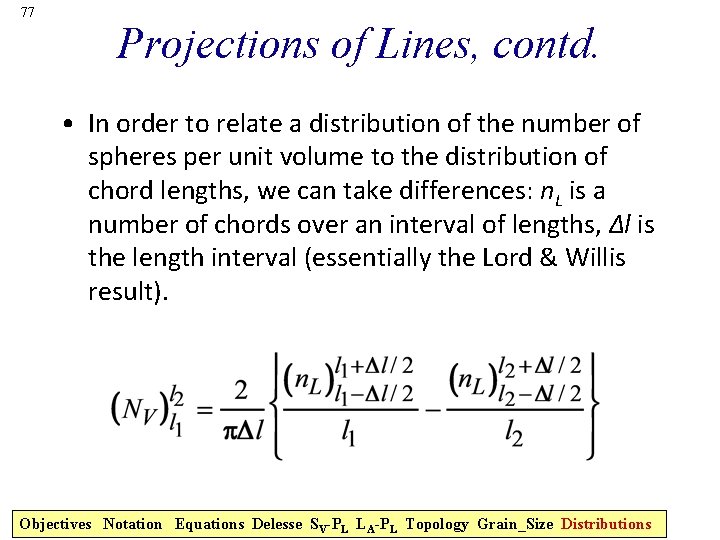
77 Projections of Lines, contd. • In order to relate a distribution of the number of spheres per unit volume to the distribution of chord lengths, we can take differences: n. L is a number of chords over an interval of lengths, ∆l is the length interval (essentially the Lord & Willis result). Objectives Notation Equations Delesse SV-PL LA-PL Topology Grain_Size Distributions

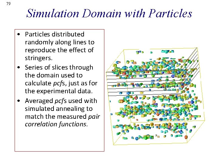
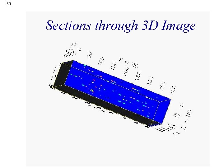
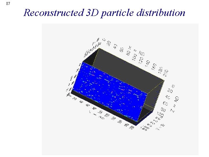
78 Artificial Digital Particle Placement • To test the system of particle analysis and generation of a 3 D digital microstructure of particles, an artificial 3 D microstructure was generated using a Cellular Automaton on a 400 x 200 x 100 regular grid (equi-axed voxels or pixels). Particles were injected along lines to mimic the stringered distributions observed in 7075. The ellipsoid axes were constrained to be aligned with the domain axes (no rotations). • This microstructure was then sectioned, as if it were a real material, the sections were analyzed, and a 3 D particle set reconstructed. • The main analytical tool employed in this technique is the (anisotropic) pair correlation function = pcf (to be explained in a later lecture). • The length units for this calculation are pixels or voxels. • See: “Three-Dimensional Characterization of Microstructure by Electron Back. Scatter Diffraction”, A. D. Rollett, S. -B. Lee, R. Campman, G. S. Rohrer, Annual Review of Materials Research, 37: 627 -658 (2007).

79 Simulation Domain with Particles • Particles distributed randomly along lines to reproduce the effect of stringers. • Series of slices through the domain used to calculate pcfs, just as for the experimental data. • Averaged pcfs used with simulated annealing to match the measured pair correlation functions.

80 Sections through 3 D Image

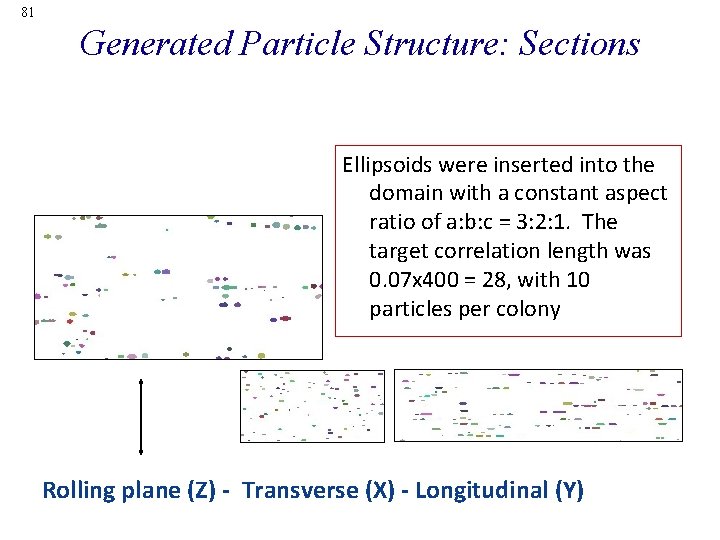
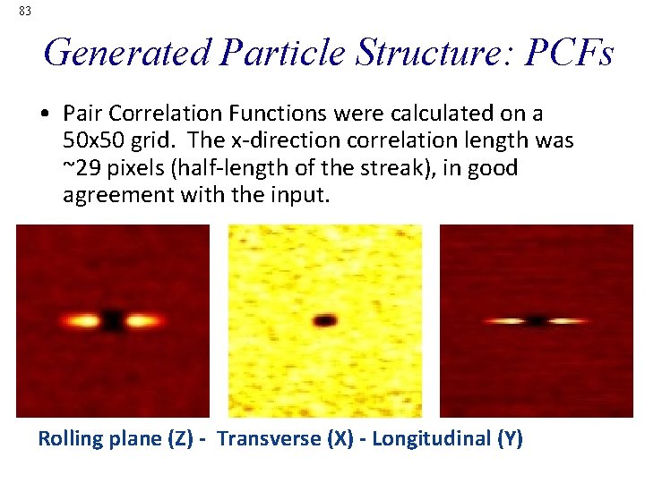
81 Generated Particle Structure: Sections Ellipsoids were inserted into the domain with a constant aspect ratio of a: b: c = 3: 2: 1. The target correlation length was 0. 07 x 400 = 28, with 10 particles per colony Rolling plane (Z) - Transverse (X) - Longitudinal (Y)

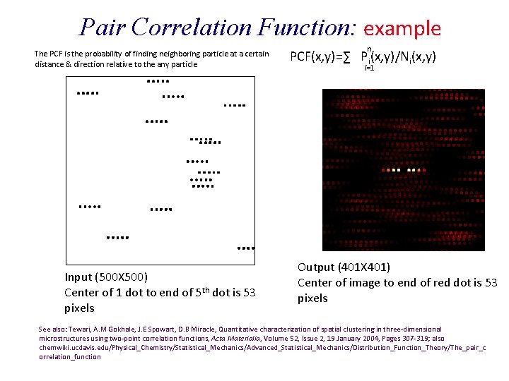
Pair Correlation Function: example The PCF is the probability of finding neighboring particle at a certain distance & direction relative to the any particle. Input (500 X 500) Center of 1 dot to end of 5 th dot is 53 pixels n PCF(x, y)=∑ Pi(x, y)/Ni(x, y) i=1 Output (401 X 401) Center of image to end of red dot is 53 pixels See also: Tewari, A. M Gokhale, J. E Spowart, D. B Miracle, Quantitative characterization of spatial clustering in three-dimensional microstructures using two-point correlation functions, Acta Materialia, Volume 52, Issue 2, 19 January 2004, Pages 307 -319; also chemwiki. ucdavis. edu/Physical_Chemistry/Statistical_Mechanics/Advanced_Statistical_Mechanics/Distribution_Function_Theory/The_pair_c orrelation_function

83 Generated Particle Structure: PCFs • Pair Correlation Functions were calculated on a 50 x 50 grid. The x-direction correlation length was ~29 pixels (half-length of the streak), in good agreement with the input. Rolling plane (Z) - Transverse (X) - Longitudinal (Y)

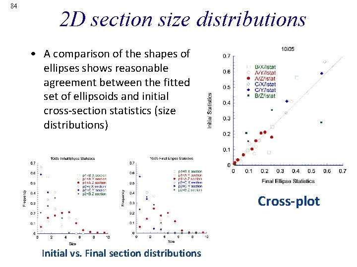
84 2 D section size distributions • A comparison of the shapes of ellipses shows reasonable agreement between the fitted set of ellipsoids and initial cross-section statistics (size distributions) Cross-plot Initial vs. Final section distributions

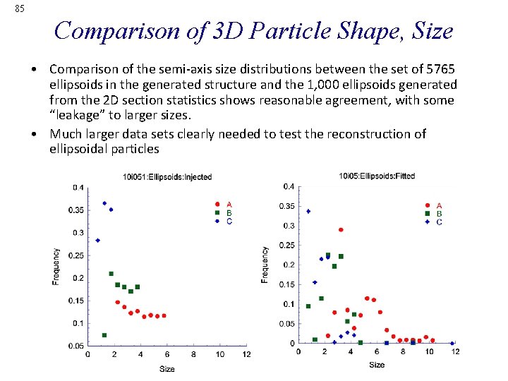
85 Comparison of 3 D Particle Shape, Size • Comparison of the semi-axis size distributions between the set of 5765 ellipsoids in the generated structure and the 1, 000 ellipsoids generated from the 2 D section statistics shows reasonable agreement, with some “leakage” to larger sizes. • Much larger data sets clearly needed to test the reconstruction of ellipsoidal particles

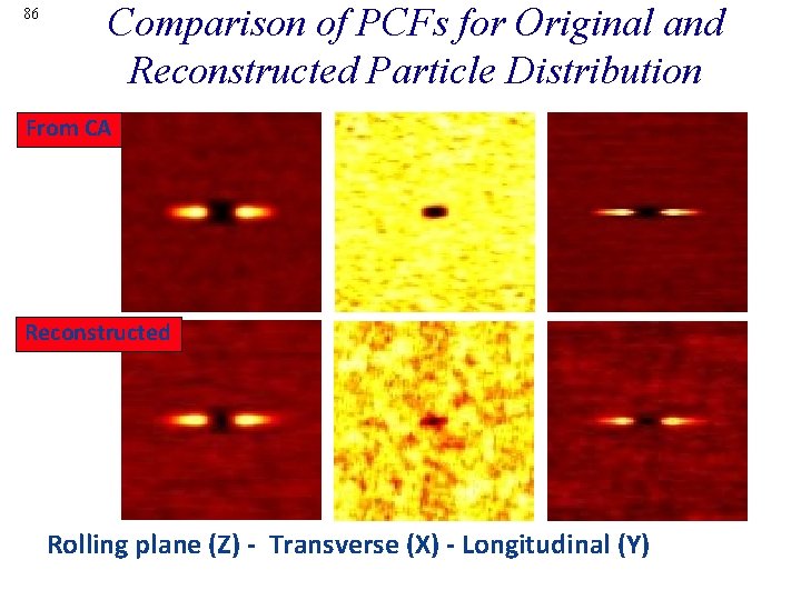
86 Comparison of PCFs for Original and Reconstructed Particle Distribution From CA Reconstructed Rolling plane (Z) - Transverse (X) - Longitudinal (Y)

87 Reconstructed 3 D particle distribution

88 Geometric Relationships • For each regular shape, whether sphere or tetrakaidecahedron, there is a set of analytical expressions that relate the dimensions of the object in 3 D to its geometry in cross section. • The following tables reproduced from Underwood summarize the available formulae. • Note the difference between projected quantities and mean intercept quantities. Example: for spheres, the projected area is the equatorial area, πr 2, whereas the mean intercept area is only 2/3 πr 2. • First slide is for bodies of revolution; second slide is for polyhedral shapes. Objectives Notation Equations Delesse SV-PL LA-PL Topology Grain_Size Distributions

89 Objectives Notation Equations Delesse SV-PL LA-PL Topology Grain_Size Distributions

90 Objectives Notation Equations Delesse SV-PL LA-PL Topology Grain_Size Distributions

91 1. 2. 3. 4. 5. 6. Questions Which set of quantities are equal to each other? The point/line/area/volume fractions. How does Buffon’s needle relate to the measurement of π? The intersection of a test line with a grid of parallel lines is related via 2 LA = π PL. Under what circumstances do we need to consider projected quantities rather than intercepts? Projected areas, e. g. , are appropriate when viewing a sample in transmission (e. g. TEM) and the feature is, say, blocking the illumination, as opposed to being viewed in cross-section. In general, do size distributions measured in 2 D show larger or smaller means than their true 3 D means? Since 2 D sections cut objects in all possible locations, the observed mean sizes are invariably smaller than the true sizes. Why are intercepts of grain boundaries with a circle sometimes used for measuring grain size? Using a circle ensures that any bias in the grain morphology does not affect the results (of grain size measurement). Why are nearest neighbor distances smaller than the mean free path for a given volume fraction and size of particle? In qualitative terms, a nearest neighbor distance is based on finding the nearest neighbor object (particle) regardless of direction, whereas a mean free path is measured in a straight line and so is unlikely to pass through the nearest neighbor (but rather a next-nearest neighbor). See also the Eqs.

92 Summary • Provided that certain assumptions about the way in which a section plane samples the 3 D microstructure are valid, statistically based relationships exist between experimental measures of points, lines and areas and various corresponding 3 D quantities.

93 Supplemental Slides • Following slides contain useful information of various kinds. 1. Definitions of statistical terms 2. Measurement of area and circumference of spheres that are instantiated on a regular grid (voxelized). 3. Verification of Stereological Relationships for (voxelized) objects on regular grids

94 1. Statistics: definitions • Population: a well defined set of individual elements or measurements (e. g. areas of grains in a micrograph). • Parameter: a numerical quantity that is defined for the population (e. g. mean grain area). • Sampling Units: non-overlapping sets of elements. The union of all sampling units is equal to the population. • Sample: a collection of sampling units taken from the population. • Estimate: a numerical approximation of a population parameter calculated from a particular sample (e. g. mean grain area calculated from a subset of the areas). • Estimator: a well-defined numerical method that describes how to calculate an estimate from a sample. • Uniform random sample: a sample taken so that all sampling units within the population possess the same probability of falling within the sample. Objectives Notation Equations Delesse SV-PL LA-PL Topology Grain_Size Distributions

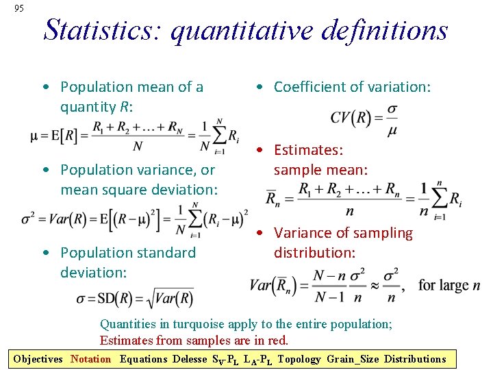
95 Statistics: quantitative definitions • Population mean of a quantity R: • Population variance, or mean square deviation: • Population standard deviation: • Coefficient of variation: • Estimates: sample mean: • Variance of sampling distribution: Quantities in turquoise apply to the entire population; Estimates from samples are in red. Objectives Notation Equations Delesse SV-PL LA-PL Topology Grain_Size Distributions

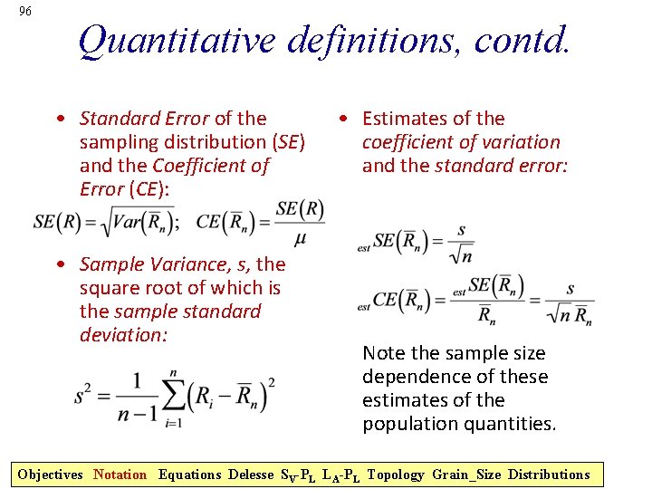
96 Quantitative definitions, contd. • Standard Error of the sampling distribution (SE) and the Coefficient of Error (CE): • Sample Variance, s, the square root of which is the sample standard deviation: • Estimates of the coefficient of variation and the standard error: Note the sample size dependence of these estimates of the population quantities. Objectives Notation Equations Delesse SV-PL LA-PL Topology Grain_Size Distributions

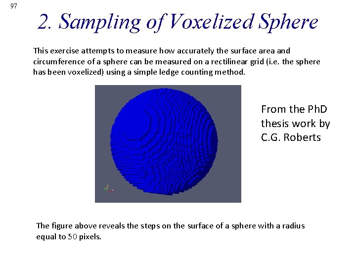
97 2. Sampling of Voxelized Sphere This exercise attempts to measure how accurately the surface area and circumference of a sphere can be measured on a rectilinear grid (i. e. the sphere has been voxelized) using a simple ledge counting method. From the Ph. D thesis work by C. G. Roberts The figure above reveals the steps on the surface of a sphere with a radius equal to 50 pixels.

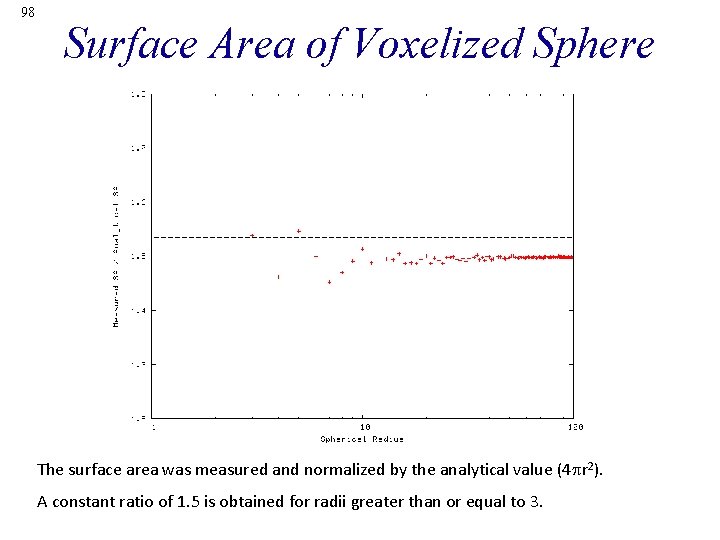
98 Surface Area of Voxelized Sphere The surface area was measured and normalized by the analytical value (4 r 2). A constant ratio of 1. 5 is obtained for radii greater than or equal to 3.

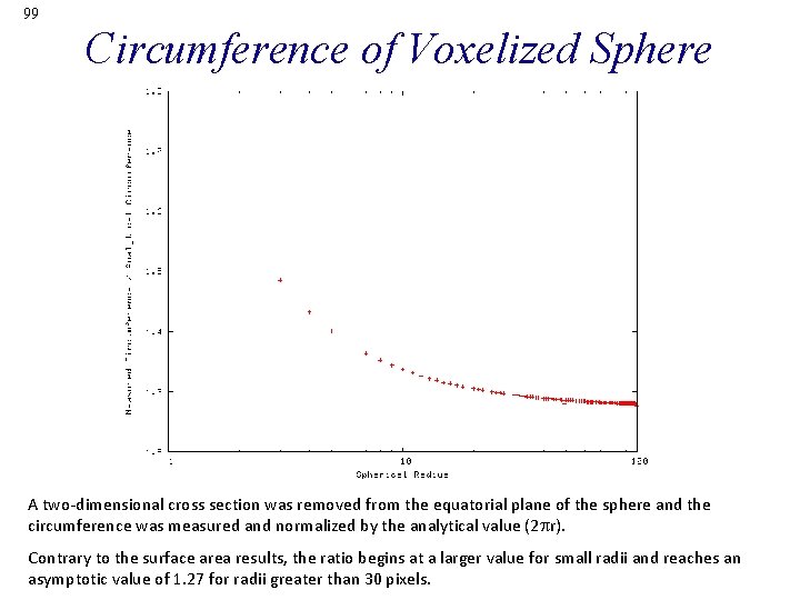
99 Circumference of Voxelized Sphere A two-dimensional cross section was removed from the equatorial plane of the sphere and the circumference was measured and normalized by the analytical value (2 r). Contrary to the surface area results, the ratio begins at a larger value for small radii and reaches an asymptotic value of 1. 27 for radii greater than 30 pixels.

100 3. Verification of Stereological Relationships Definition: Stereology is the interpretation of three-dimensional structures based on twodimensional observations. The relationships between lower and higher dimensionality are primarily mathematical in nature. Practicality: A majority of experimental investigations involve destructive evaluation of the specimen wherein the researcher measures the parameter of interest on a crosssectional area; therefore, stereology provides the link between the planar and volumetric quantities.

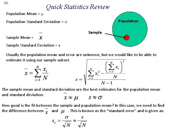
101 Quick Statistics Review Population Mean = Population Standard Deviation = Sample Mean = Sample Standard Deviation = s Usually the population mean and error are unknown, but we would like to be able to estimate it using our sample subset. The sample mean and standard deviation are the best estimates for the population mean and standard deviation. How good is the fit between the sample and population mean? In this case, we need to find the difference between and . This is known as the “standard error” and is given as:

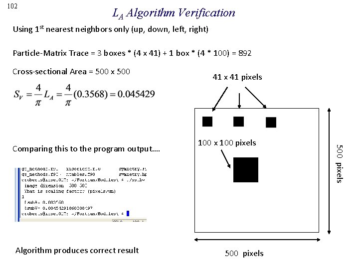
102 LA Algorithm Verification Using 1 st nearest neighbors only (up, down, left, right) Particle-Matrix Trace = 3 boxes * (4 x 41) + 1 box * (4 * 100) = 892 Cross-sectional Area = 500 x 500 Algorithm produces correct result 100 x 100 pixels 500 pixels Comparing this to the program output…. 41 x 41 pixels

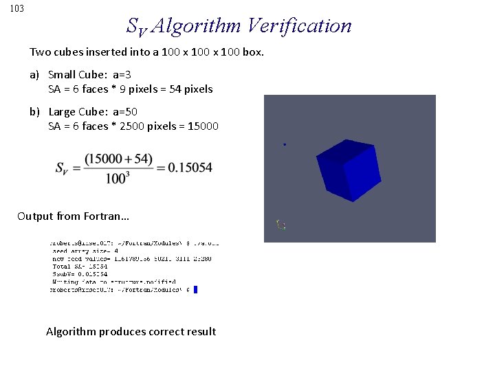
103 SV Algorithm Verification Two cubes inserted into a 100 x 100 box. a) Small Cube: a=3 SA = 6 faces * 9 pixels = 54 pixels b) Large Cube: a=50 SA = 6 faces * 2500 pixels = 15000 Output from Fortran… Algorithm produces correct result

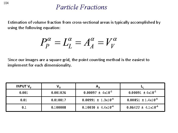
104 Particle Fractions Estimation of volume fraction from cross-sectional areas is typically accomplished by using the following equation: Since our images are a square grid, the point counting method is the easiest to implement for each dimensionality. INPUT VV VV AA LL 0. 001026 0. 00097 ± 4 x 10 -5 0. 00091 ± 4 x 10 -5 0. 010017 0. 00991 ± 1. 3 x 10 -4 0. 00851 ± 1. 4 x 10 -4 0. 100008 0. 10030 ± 4. 4 x 10 -4 0. 06422 ± 4. 1 x 10 -4

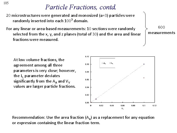
105 Particle Fractions, contd. 20 microstructures were generated and monosized (a=3) particles were randomly inserted into each 1003 domain. For any linear or area-based measurements: 10 sections were randomly selected from the x, y, and z planes (total of 30) and the area and linear fractions were measured. 600 measurements At low volume fractions, the agreement among all three parameters is very close; however, the LL parameter deviates significantly from the AA and VV values are larger particle fractions. Recommendation: Use the area fraction (AA) as a replacement for any equation or expression containing the linear fraction term.

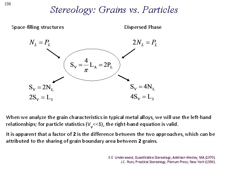
106 Stereology: Grains vs. Particles Space-filling structures Dispersed Phase When we analyze the grain characteristics in typical metal alloys, we will use the left-hand relationships; for particle statistics (VV<<1), the right-hand equation is valid. It is apparent that a factor of 2 is the difference between the two approaches, which can be attributed to the sharing of grain boundary area between 2 grains. E. E. Underwood, Quantitative Stereology, Addison-Wesley, MA (1970). J. C. Russ, Practical Stereology, Plenum Press, New York (1986).

107 Stereology: LA and SV Since most experimental studies involve two-dimensional statistical analyses, one inevitably will need to apply stereology to obtain a 3 D parameter. Quantities highlighted with circles are easily measured on 2 D planes. We are interested in finding out how accurate the highlighted relationship is using computer generated three-dimensional structures.

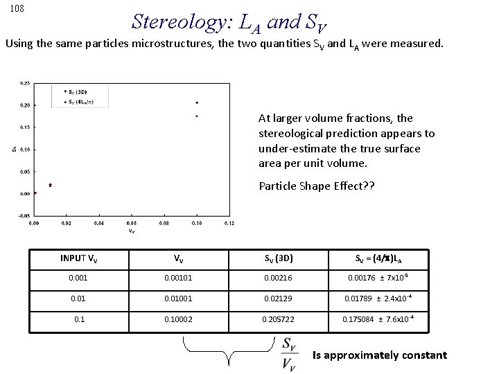
108 Stereology: LA and SV Using the same particles microstructures, the two quantities SV and LA were measured. At larger volume fractions, the stereological prediction appears to under-estimate the true surface area per unit volume. Particle Shape Effect? ? INPUT VV VV SV (3 D) SV = (4/ )LA 0. 00101 0. 00216 0. 00176 ± 7 x 10 -5 0. 01001 0. 02129 0. 01789 ± 2. 4 x 10 -4 0. 10002 0. 205722 0. 175084 ± 7. 6 x 10 -4 Is approximately constant

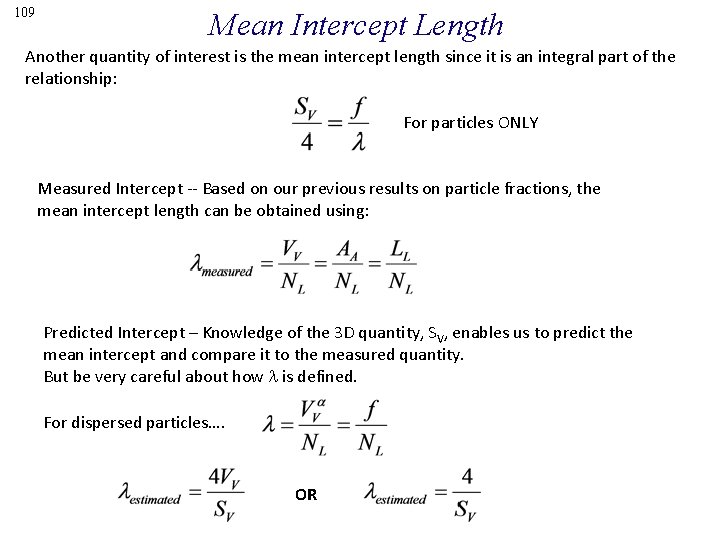
109 Mean Intercept Length Another quantity of interest is the mean intercept length since it is an integral part of the relationship: For particles ONLY Measured Intercept -- Based on our previous results on particle fractions, the mean intercept length can be obtained using: Predicted Intercept – Knowledge of the 3 D quantity, SV, enables us to predict the mean intercept and compare it to the measured quantity. But be very careful about how is defined. For dispersed particles…. OR

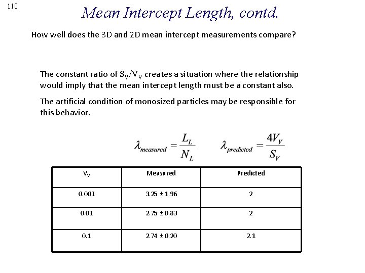
110 Mean Intercept Length, contd. How well does the 3 D and 2 D mean intercept measurements compare? The constant ratio of SV/VV creates a situation where the relationship would imply that the mean intercept length must be a constant also. The artificial condition of monosized particles may be responsible for this behavior. VV Measured Predicted 0. 001 3. 25 ± 1. 96 2 0. 01 2. 75 ± 0. 83 2 0. 1 2. 74 ± 0. 20 2. 1

111 Conclusions • The area fraction measurements provide an accurate estimate of the threedimensional volume fraction for VV 0. 1 while the line fraction significantly underestimates the true 3 D quantity. • Line trace per unit area under-estimates the surface area per unit volume for volume fractions above 1 percent. • The predicted mean intercept length cannot be used as a substitute for the measurement of the mean intercept length.