Texture Key issue representing texture Texture based matching

Texture • Key issue: representing texture – Texture based matching • little is known – Texture segmentation • key issue: representing texture – Texture synthesis • useful; also gives some insight into quality of representation – Shape from texture • cover superficially

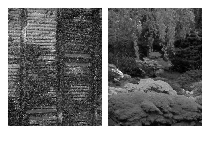
Representing textures • Textures are made up of quite stylised subelements, repeated in meaningful ways • Representation: – find the subelements, and represent their statistics • But what are the subelements, and how do we find them? – recall normalized correlation – find subelements by applying filters, looking at the magnitude of the response • What filters? – experience suggests spots and oriented bars at a variety of different scales – details probably don’t matter • What statistics? – within reason, the more the merrier. – At least, mean and standard deviation – better, various conditional histograms.

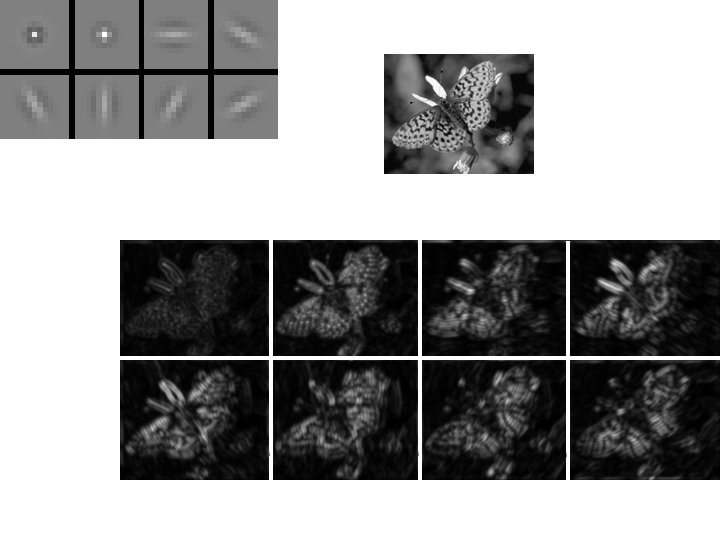
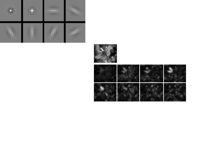
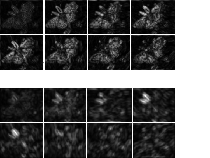
Gabor filters at different scales and spatial frequencies top row shows anti-symmetric (or odd) filters, bottom row the symmetric (or even) filters.

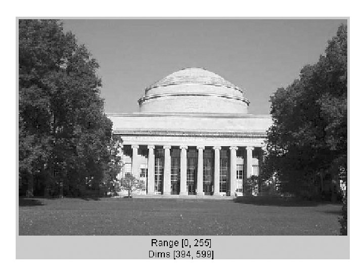
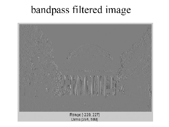
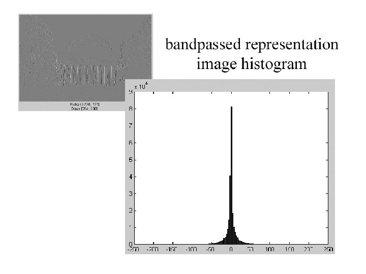
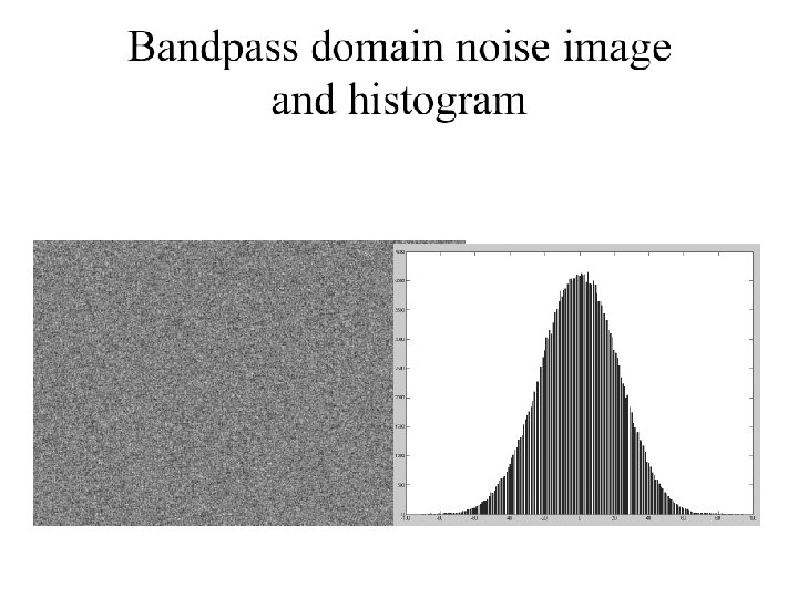
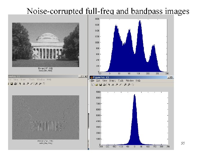
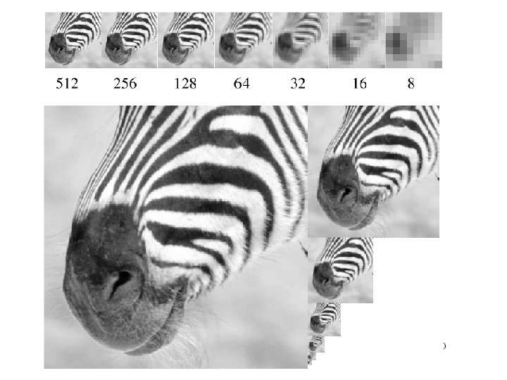
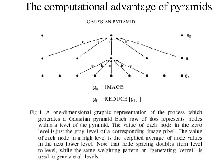
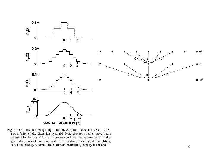
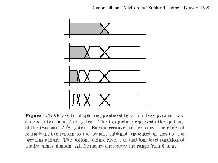
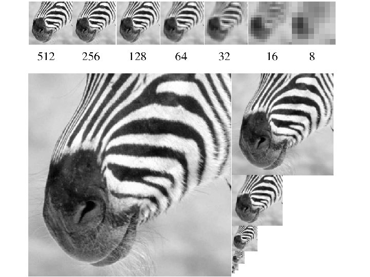
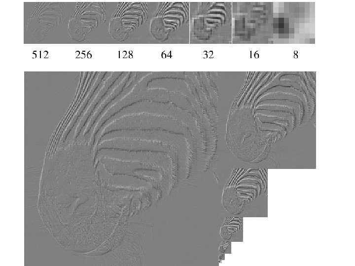
The Laplacian Pyramid • Synthesis – preserve difference between upsampled Gaussian pyramid level and Gaussian pyramid level – band pass filter - each level represents spatial frequencies (largely) unrepresented at other levels • Analysis – reconstruct Gaussian pyramid, take top layer

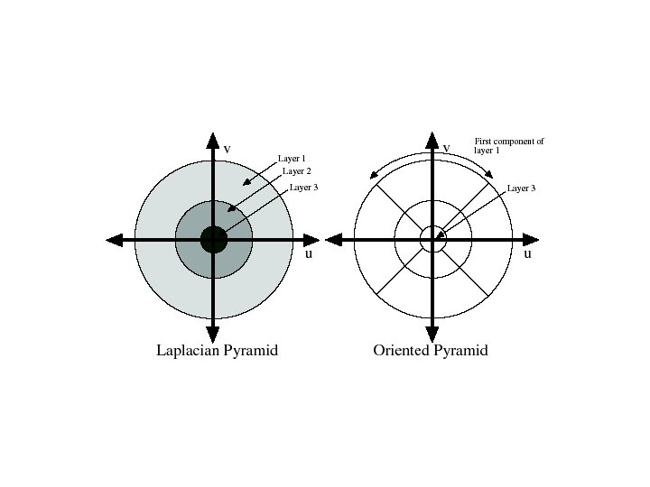
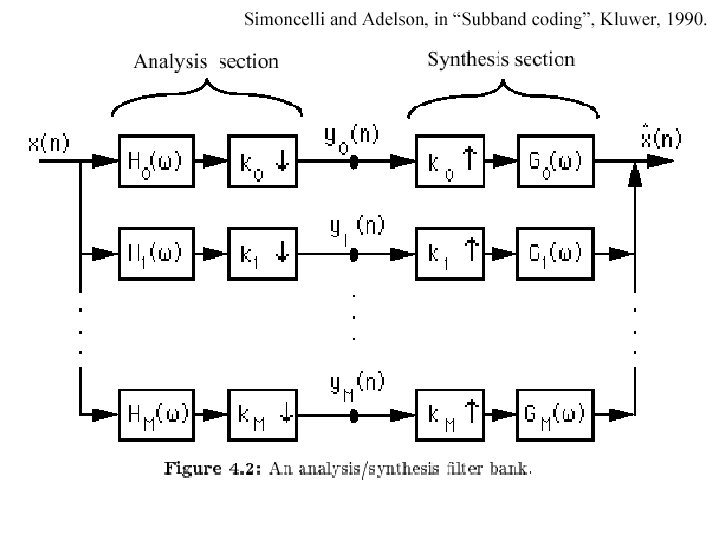
Oriented pyramids • Laplacian pyramid is orientation independent • Apply an oriented filter to determine orientations at each layer – by clever filter design, we can simplify synthesis – this represents image information at a particular scale and orientation

Steerable Pyramids http: //www. cis. upenn. edu/~eero/steerpyr. html

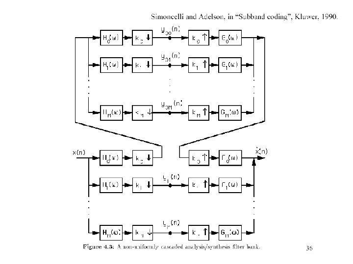
Reprinted from “Shiftable Multi. Scale Transforms, ” by Simoncelli et al. , IEEE Transactions

Analysis

synthesis

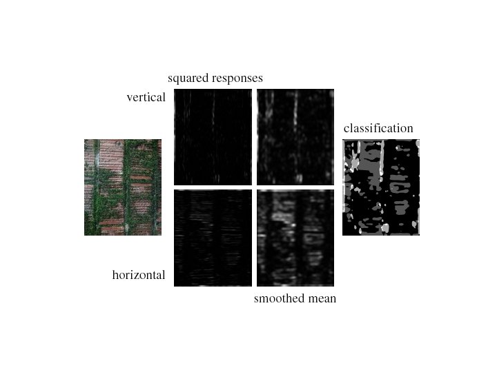
Final texture representation • Form an oriented pyramid (or equivalent set of responses to filters at different scales and orientations). • Square the output • Take statistics of squared responses – – e. g. mean of each filter output (are there lots of spots) std of each filter output Histogram of responses mean of one scale conditioned on other scale having a particular range of values (e. g. are the spots in straight rows? )

Texture synthesis • Use image as a source of probability model • Choose pixel values by matching neighbourhood, then filling in • Matching process – look at pixel differences – count only synthesized pixels

Figure from Texture Synthesis by Non-parametric Sampling, A. Efros and T. K. Leung, Proc.

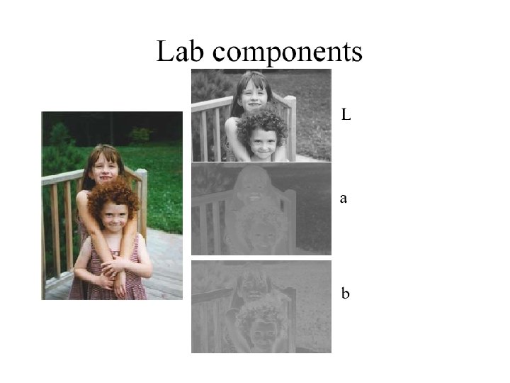
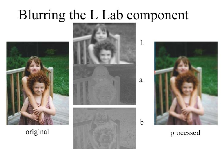
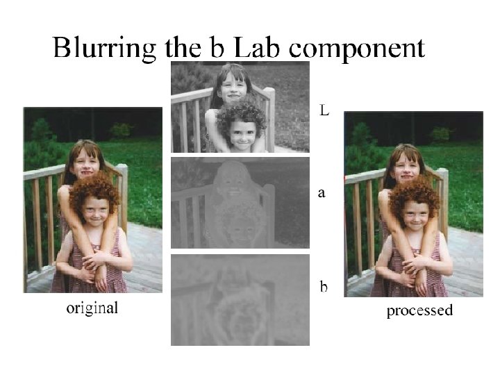
RGB to Lab color space • • [ X ] [ [ Y ] = [ [ Z ] [ 0. 412453 0. 212671 0. 019334 0. 357580 0. 189423 ] [ R ] 0. 715160 0. 072169 ] * [ G ] 0. 119193 0. 950227 ] [ B ]. CIE 1976 L*a*b* is based directly on CIE XYZ and is an attampt to linearize the perceptibility of color differences. The non-linear relations for L*, and b* are intended to mimic the logarithmic response of the eye. Coloring information is referred to the color of the white point of the system, subscript n. • L* = 116 * (Y/Yn)1/3 - 16 • L* = 903. 3 * Y/Yn for Y/Yn > 0. 008856 otherwise • a* = 500 * ( f(X/Xn) - f(Y/Yn) ) • b* = 200 * ( f(Y/Yn) - f(Z/Zn) )

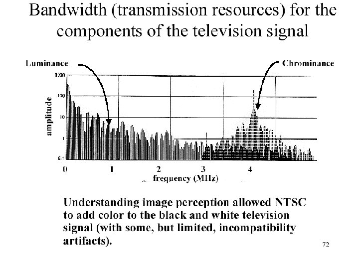
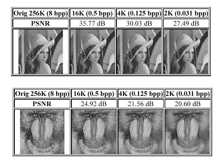
Compression

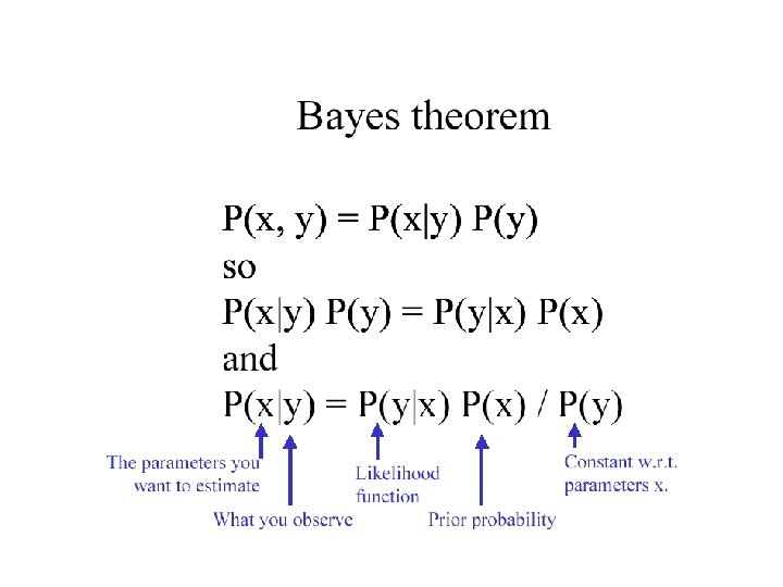
Mr. Dupont is a professional wine taster. When given a French wine, he will identify it with probability 0. 9 correctly as French, and will mistake it for a Californian wine with probability 0. 1. When given a Californian wine, he will identify it with probability 0. 8 correctly as Californian, and will mistake it for a French wine with probability 0. 2. Suppose that Mr. Dupont is given ten unlabelled glasses of wine, three with French and seven with Californian wines. He randomly picks a glass, tries the wine, and solemnly says: "French". What is the probability that the wine he tasted was Californian?

Mr. Dupont is a professional wine taster. When given a French wine, he will identify it with probability 0. 9 correctly as French, and will mistake it for a Californian wine with probability 0. 1. When given a Californian wine, he will identify it with probability 0. 8 correctly as Californian, and will mistake it for a French wine with probability 0. 2. Suppose that Mr. Dupont is given ten unlabelled glasses of wine, three with French and seven with Californian wines. He randomly picks a glass, tries the wine, and solemnly says: "French". What is the probability that the wine he tasted was Californian? Rf F 0. 9 C 0. 1 Rc 0. 2 0. 8 P(F) = 0. 3; P(C) = 0. 7; P(C|Rf) = P(Rf|C) p( C )/P(Rf) S = 0. 1*0. 7/ w P(Rf |w)p(w) = 0. 1*0. 7/(0. 9*0. 3+0. 1*0. 7) = 0. 21 = 0. 1*0. 7/0. 34 = 0. 21

“You must choose, but Choose Wisely” • Given only probabilities, can we minimize the number of errors we make? • Given: responses Ri, categories Ci, current category c, data x • To Minimize error: – Decide Ri if P(Ci | x) > P(Ck | x) for all i≠k P( x | Ci) P(Ci ) > P(x | Ck ) P( x | Ci)/ P(x | Ck ) > P(Ck ) / P(Ci ) P( x | Ci)/ P(x | Ck ) > T Optimal classifications always involve hard boundaries

Horse Segmentation

P(horse) = 0. 04 P(background) = 0. 96 • P(red|horse) P(red|background)

Now evaluate