Texture Texture Texture is an innate property of

Texture

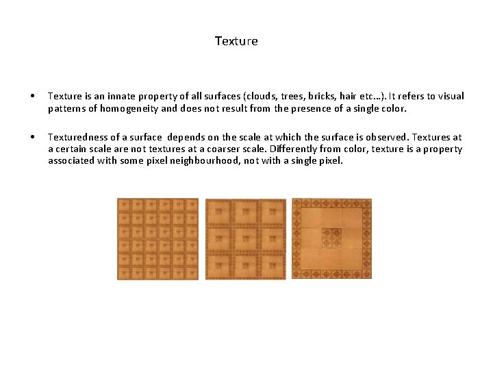
Texture • Texture is an innate property of all surfaces (clouds, trees, bricks, hair etc…). It refers to visual patterns of homogeneity and does not result from the presence of a single color. • Texturedness of a surface depends on the scale at which the surface is observed. Textures at a certain scale are not textures at a coarser scale. Differently from color, texture is a property associated with some pixel neighbourhood, not with a single pixel.

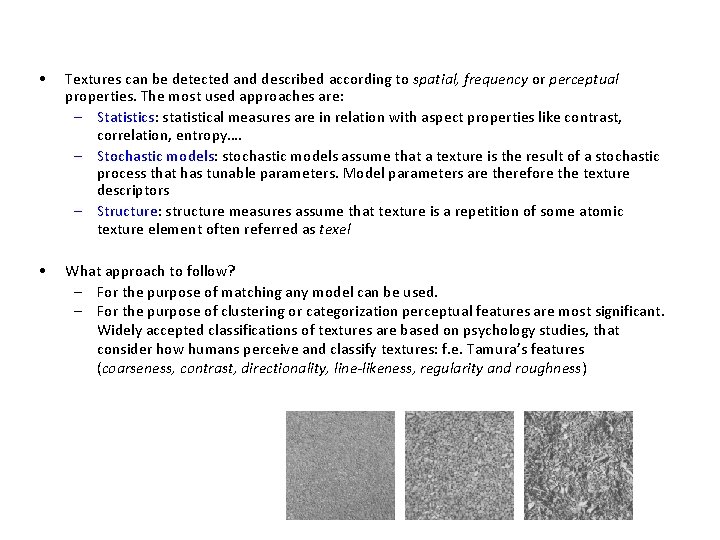
• Textures can be detected and described according to spatial, frequency or perceptual properties. The most used approaches are: – Statistics: statistical measures are in relation with aspect properties like contrast, correlation, entropy…. – Stochastic models: stochastic models assume that a texture is the result of a stochastic process that has tunable parameters. Model parameters are therefore the texture descriptors – Structure: structure measures assume that texture is a repetition of some atomic texture element often referred as texel • What approach to follow? – For the purpose of matching any model can be used. – For the purpose of clustering or categorization perceptual features are most significant. Widely accepted classifications of textures are based on psychology studies, that consider how humans perceive and classify textures: f. e. Tamura’s features (coarseness, contrast, directionality, line-likeness, regularity and roughness)

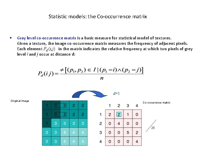
Statistic models: the Co-occurrence matrix • Gray level co-occurrence matrix is a basic measure for statistical model of textures. Given a texture, the image co-occurrence matrix measures the frequency of adjacent pixels. Each element Pd (i, j) in the matrix indicates the relative frequency at which two pixels of grey level i and j occur at distance d: d=1 Original image Co-occurrence matrix 25

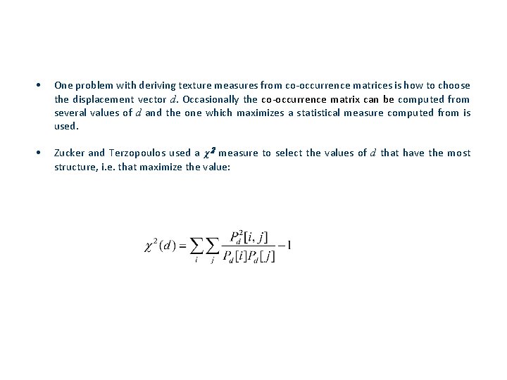
• One problem with deriving texture measures from co-occurrence matrices is how to choose the displacement vector d. Occasionally the co-occurrence matrix can be computed from several values of d and the one which maximizes a statistical measure computed from is used. • Zucker and Terzopoulos used a χ 2 measure to select the values of d that have the most structure, i. e. that maximize the value:

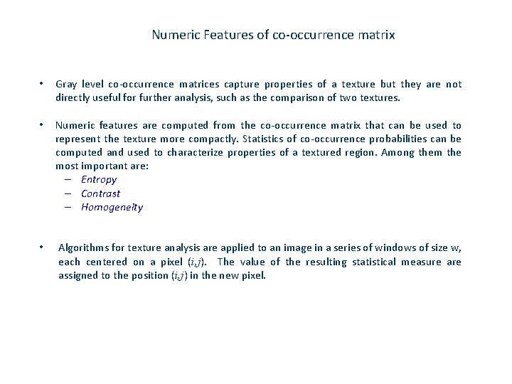
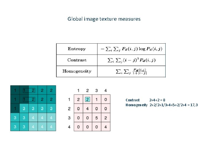
Numeric Features of co-occurrence matrix • Gray level co-occurrence matrices capture properties of a texture but they are not directly useful for further analysis, such as the comparison of two textures. • Numeric features are computed from the co-occurrence matrix that can be used to represent the texture more compactly. Statistics of co-occurrence probabilities can be computed and used to characterize properties of a textured region. Among them the most important are: – Entropy – Contrast – Homogeneity • Algorithms for texture analysis are applied to an image in a series of windows of size w, each centered on a pixel (i, j). The value of the resulting statistical measure assigned to the position (i, j) in the new pixel.

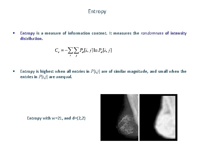
Entropy • Entropy is a measure of information content. It measures the randomness of intensity distribution. • Entropy is highest when all entries in P[i, j] are of similar magnitude, and small when the entries in P[i, j] are unequal. Entropy with w=21, and d=(2, 2)

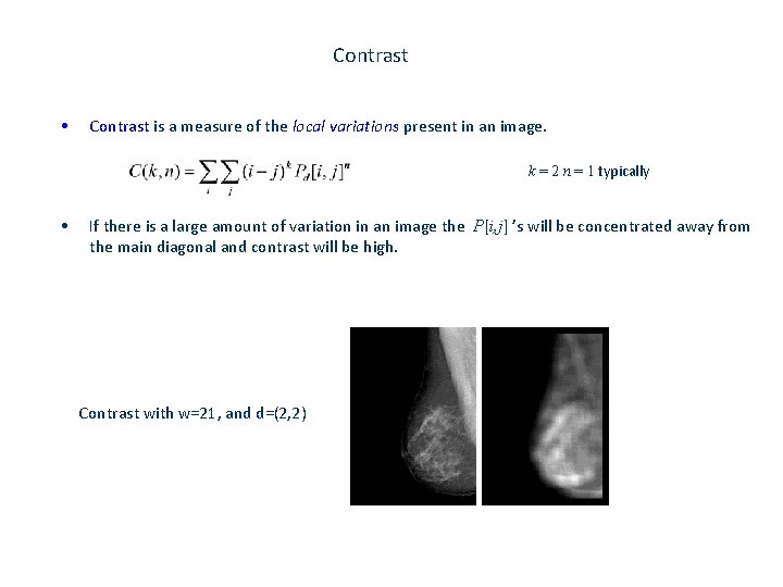
Contrast • Contrast is a measure of the local variations present in an image. k = 2 n = 1 typically • If there is a large amount of variation in an image the P[i, j] ’s will be concentrated away from the main diagonal and contrast will be high. Contrast with w=21, and d=(2, 2)

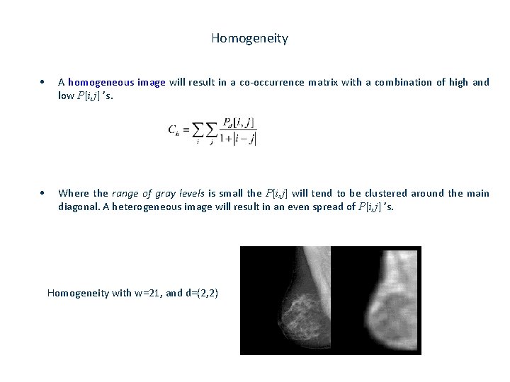
Homogeneity • A homogeneous image will result in a co-occurrence matrix with a combination of high and low P[i, j] ’s. • Where the range of gray levels is small the P[i, j] will tend to be clustered around the main diagonal. A heterogeneous image will result in an even spread of P[i, j] ’s. Homogeneity with w=21, and d=(2, 2)

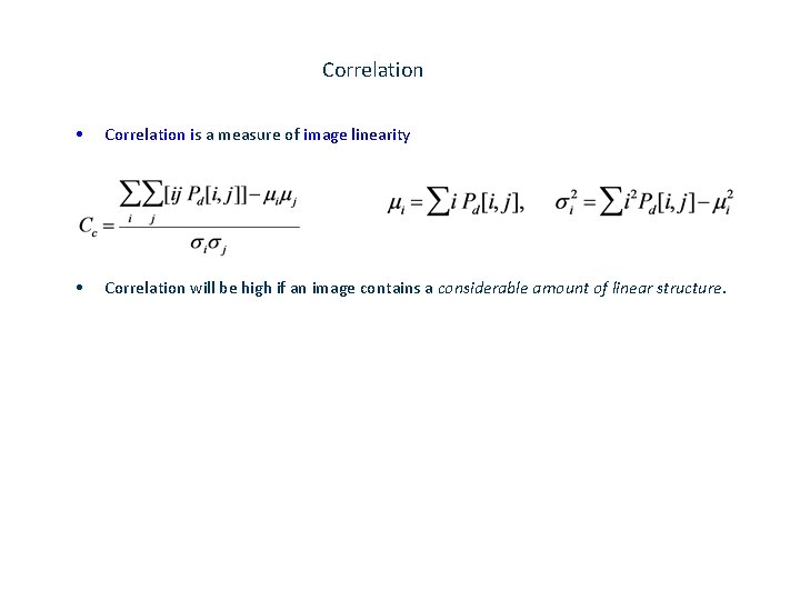
Correlation • Correlation is a measure of image linearity • Correlation will be high if an image contains a considerable amount of linear structure.

Global image texture measures Contrast 2+4+2 = 8 Homogeneity 2+2/2+1/3+4+5+2/2+4 = 17, 3

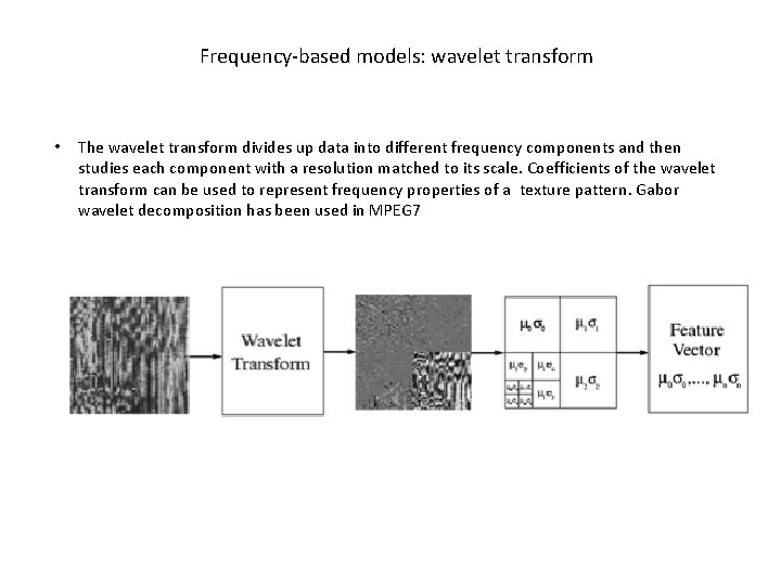
Frequency-based models: wavelet transform • The wavelet transform divides up data into different frequency components and then studies each component with a resolution matched to its scale. Coefficients of the wavelet transform can be used to represent frequency properties of a texture pattern. Gabor wavelet decomposition has been used in MPEG 7

Perceptual models: Tamura’s features • Tamura’s features are based on psychophysical studies of the characterizing elements that are perceived in textures by humans : – Contrast – Directionality – Coarseness – Linelikeness – Regularity – Roughness

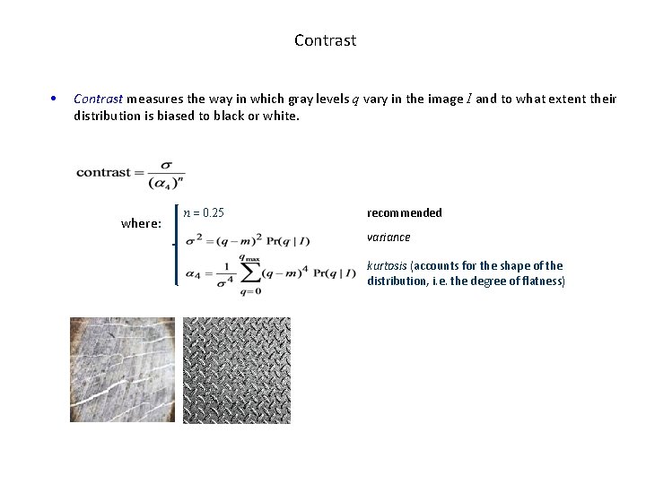
Contrast • Contrast measures the way in which gray levels q vary in the image I and to what extent their distribution is biased to black or white. where: n = 0. 25 recommended variance kurtosis (accounts for the shape of the distribution, i. e. the degree of flatness)

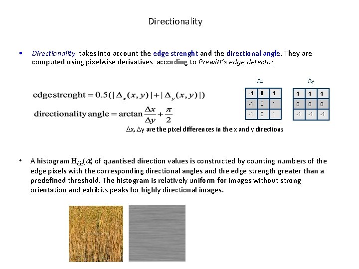
Directionality • Directionality takes into account the edge strenght and the directional angle. They are computed using pixelwise derivatives according to Prewitt’s edge detector x y -1 0 1 1 -1 0 0 0 -1 0 1 -1 -1 -1 x, y are the pixel differences in the x and y directions • A histogram Hdir(a) of quantised direction values is constructed by counting numbers of the edge pixels with the corresponding directional angles and the edge strength greater than a predefined threshold. The histogram is relatively uniform for images without strong orientation and exhibits peaks for highly directional images.

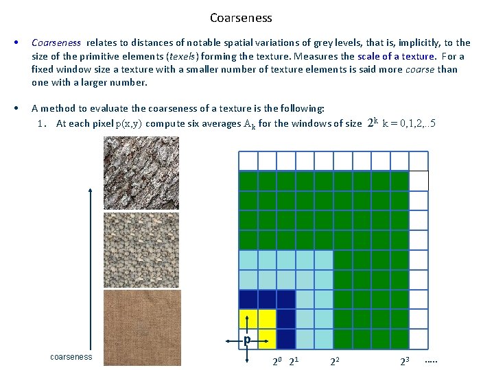
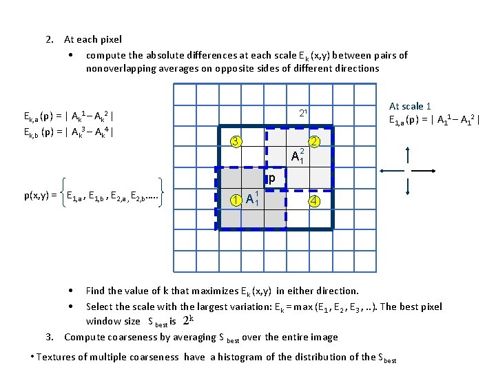
Coarseness • Coarseness relates to distances of notable spatial variations of grey levels, that is, implicitly, to the size of the primitive elements (texels) forming the texture. Measures the scale of a texture. For a fixed window size a texture with a smaller number of texture elements is said more coarse than one with a larger number. • A method to evaluate the coarseness of a texture is the following: 1. At each pixel p(x, y) compute six averages Ak for the windows of size 2 k k = 0, 1, 2, . . 5 p coarseness 20 21 22 23 …. .

2. At each pixel • compute the absolute differences at each scale Ek (x, y) between pairs of nonoverlapping averages on opposite sides of different directions Ek, a (p) = | Ak 1 – Ak 2 | Ek, b (p) = | Ak 3 – Ak 4 | At scale 1 E 1, a (p) = | A 11 – A 12 | 21 3 2 2 A 1 p p(x, y) = E 1, a , E 1, b , E 2, a , E 2, b…. . 1 1 A 1 4 • • Find the value of k that maximizes Ek (x, y) in either direction. Select the scale with the largest variation: Ek = max (E 1 , E 2 , E 3 , . . ). The best pixel window size S best is 2 k 3. Compute coarseness by averaging S best over the entire image • Textures of multiple coarseness have a histogram of the distribution of the Sbest

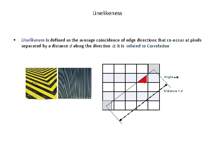
Linelikeness • Linelikeness is defined as the average coincidence of edge directions that co-occur at pixels separated by a distance d along the direction a. it is related to Correlation Angle = a Distance = d

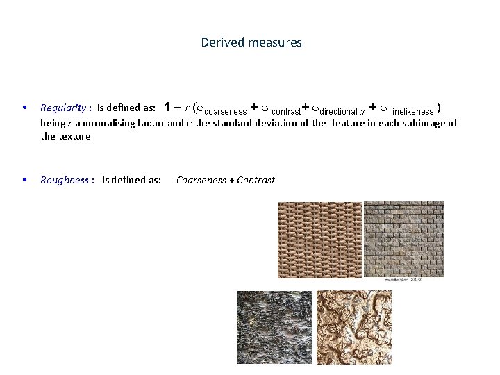
Derived measures • Regularity : is defined as: 1 – r (scoarseness + s contrast+ sdirectionality + s linelikeness ) being r a normalising factor and s the standard deviation of the feature in each subimage of the texture • Roughness : is defined as: Coarseness + Contrast