Simple Linear Regression Terminology Moments Skewness Kurtosis Analysis

Simple Linear Regression

Terminology Moments, Skewness, Kurtosis Analysis of variance ANOVA Response (dependent) variable Explanatory (independent) variable Linear regression model 　　　　　 Method of least squares Normal equation sum of squares, Error SSE sum of squares, Regression SSR sum of squares, Total SST Coefficient of Determination R 2 F-value P-value, t-test, F-test, p-test Homoscedasticity heteroscedasticity 　 　 　　　　　

Contents • 18. 0 Normal distribution and terms • 18. 1 An Example • 18. 2 The Simple Linear Regression Model • 18. 3 Estimation: The Method of Least Squares • 18. 4 Error Variance and the Standard Errors of Regression • • • Estimators 18. 5 Confidence Intervals for the Regression Parameters 18. 6 Hypothesis Tests about the Regression Relationship 18. 7 How Good is the Regression? 18. 8 Analysis of Variance Table and an F Test of the Regression Model 18. 9 Residual Analysis 18. 10 Prediction Interval and Confidence Interval

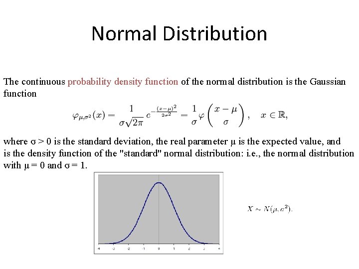
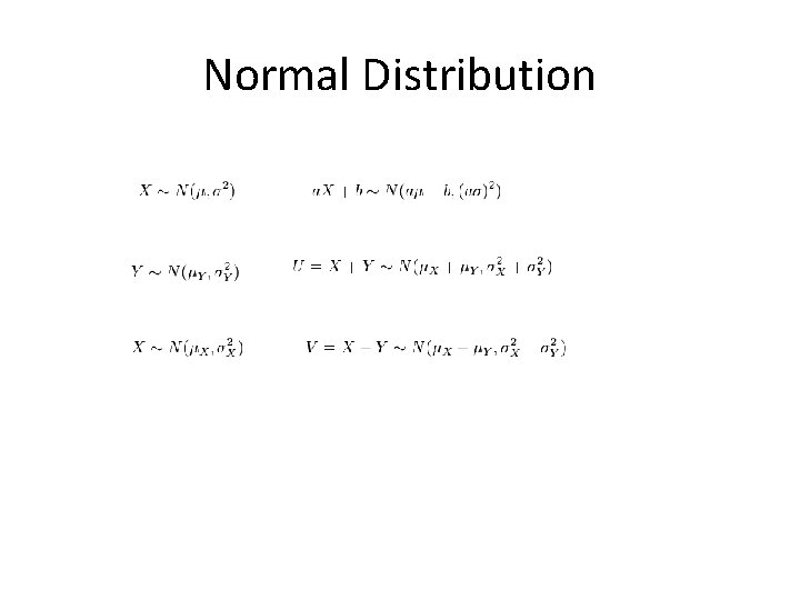
Normal Distribution The continuous probability density function of the normal distribution is the Gaussian function where σ > 0 is the standard deviation, the real parameter μ is the expected value, and is the density function of the "standard" normal distribution: i. e. , the normal distribution with μ = 0 and σ = 1.

Normal Distribution

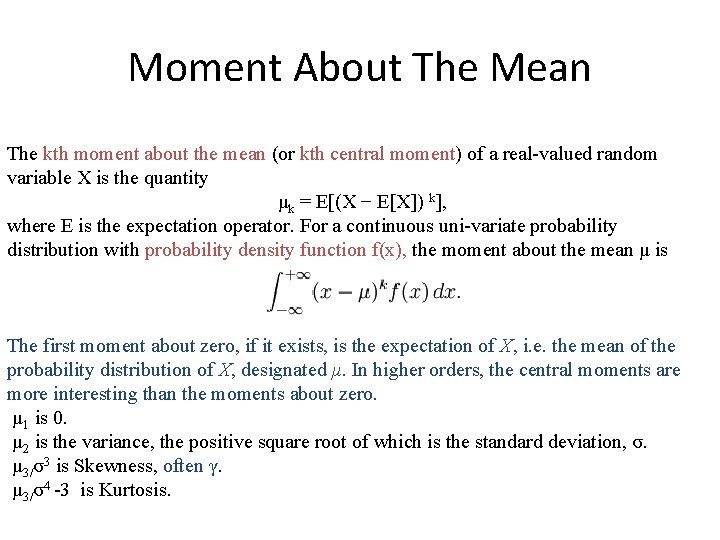
Moment About The Mean The kth moment about the mean (or kth central moment) of a real-valued random variable X is the quantity μk = E[(X − E[X]) k], where E is the expectation operator. For a continuous uni-variate probability distribution with probability density function f(x), the moment about the mean μ is The first moment about zero, if it exists, is the expectation of X, i. e. the mean of the probability distribution of X, designated μ. In higher orders, the central moments are more interesting than the moments about zero. μ 1 is 0. μ 2 is the variance, the positive square root of which is the standard deviation, σ. μ 3/σ3 is Skewness, often γ. μ 3/σ4 -3 is Kurtosis.

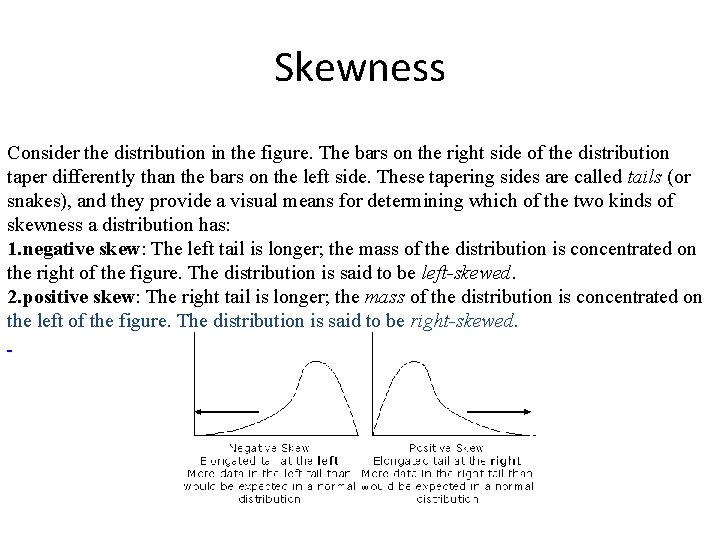
Skewness Consider the distribution in the figure. The bars on the right side of the distribution taper differently than the bars on the left side. These tapering sides are called tails (or snakes), and they provide a visual means for determining which of the two kinds of skewness a distribution has: 1. negative skew: The left tail is longer; the mass of the distribution is concentrated on the right of the figure. The distribution is said to be left-skewed. 2. positive skew: The right tail is longer; the mass of the distribution is concentrated on the left of the figure. The distribution is said to be right-skewed.

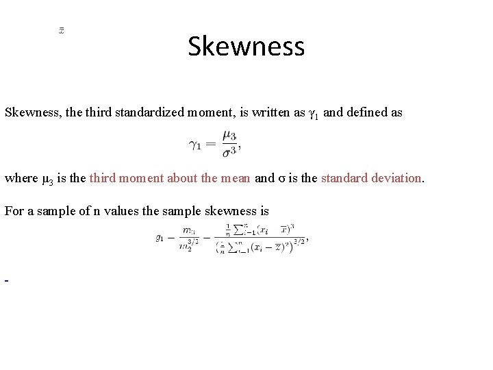
Skewness, the third standardized moment, is written as γ 1 and defined as where μ 3 is the third moment about the mean and σ is the standard deviation. For a sample of n values the sample skewness is

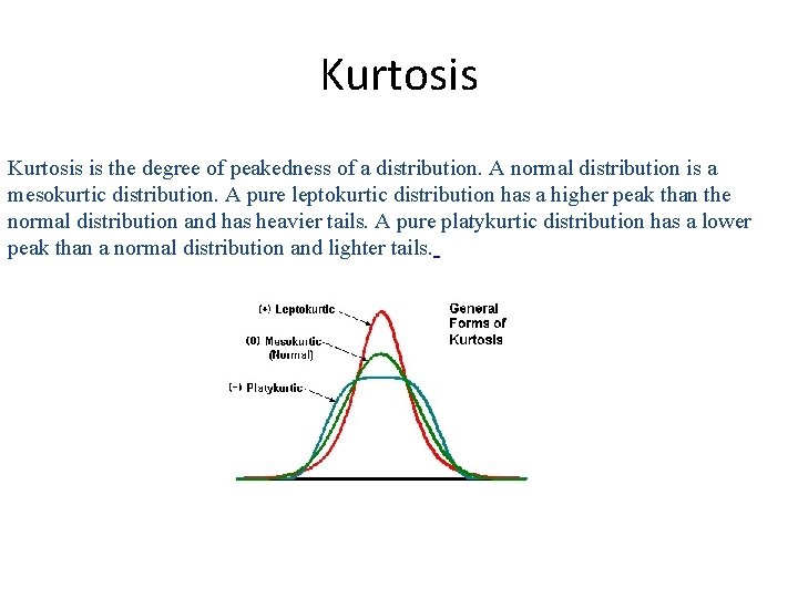
Kurtosis is the degree of peakedness of a distribution. A normal distribution is a mesokurtic distribution. A pure leptokurtic distribution has a higher peak than the normal distribution and has heavier tails. A pure platykurtic distribution has a lower peak than a normal distribution and lighter tails.

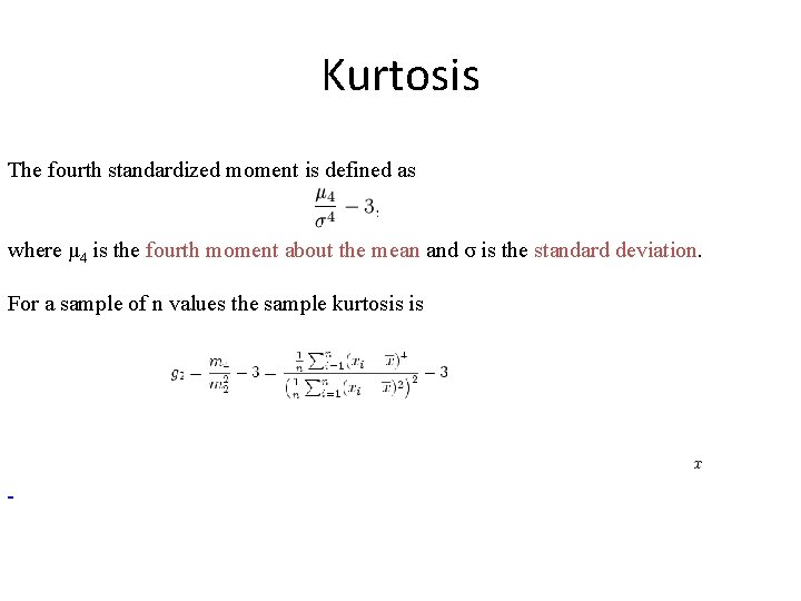
Kurtosis The fourth standardized moment is defined as where μ 4 is the fourth moment about the mean and σ is the standard deviation. For a sample of n values the sample kurtosis is

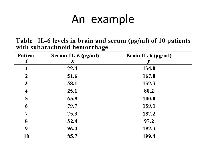
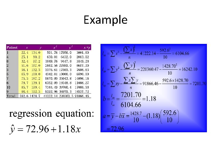
An example Table IL-6 levels in brain and serum (pg/ml) of 10 patients with subarachnoid hemorrhage Patient i 1 2 3 4 5 6 7 8 9 10 Serum IL-6 (pg/ml) x 22. 4 51. 6 58. 1 25. 1 65. 9 79. 7 75. 3 32. 4 96. 4 85. 7 Brain IL-6 (pg/ml) y 134. 0 167. 0 132. 3 80. 2 100. 0 139. 1 187. 2 97. 2 192. 3 199. 4

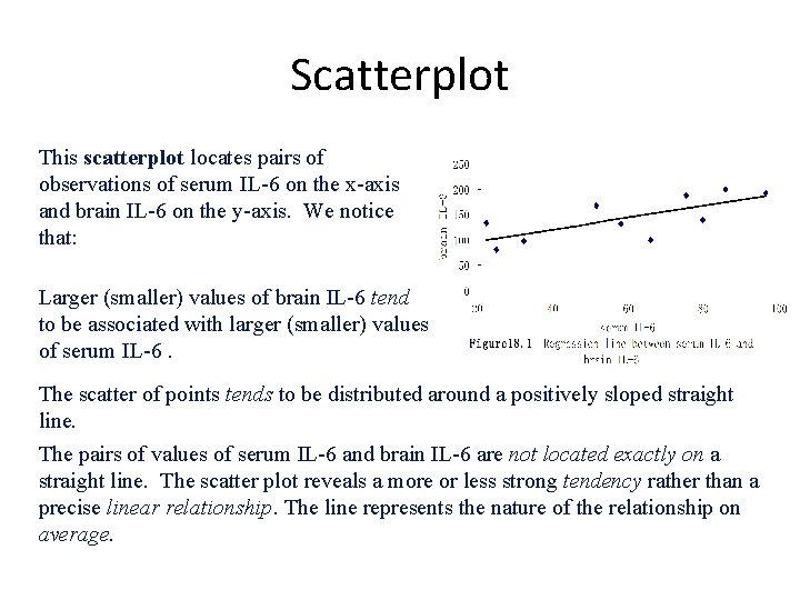
Scatterplot This scatterplot locates pairs of observations of serum IL-6 on the x-axis and brain IL-6 on the y-axis. We notice that: Larger (smaller) values of brain IL-6 tend to be associated with larger (smaller) values of serum IL-6. The scatter of points tends to be distributed around a positively sloped straight line. The pairs of values of serum IL-6 and brain IL-6 are not located exactly on a straight line. The scatter plot reveals a more or less strong tendency rather than a precise linear relationship. The line represents the nature of the relationship on average.

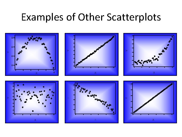
Examples of Other Scatterplots 0 Y Y Y 0 0 X X X Y Y Y X X X

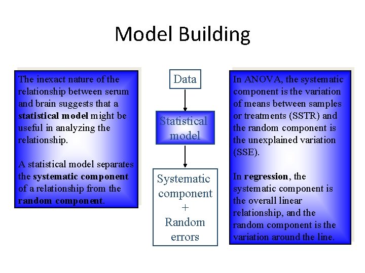
Model Building The inexact nature of the relationship between serum and brain suggests that a statistical model might be useful in analyzing the relationship. A statistical model separates the systematic component of a relationship from the random component. Data Statistical model Systematic component + Random errors In ANOVA, the systematic component is the variation of means between samples or treatments (SSTR) and the random component is the unexplained variation (SSE). In regression, the systematic component is the overall linear relationship, and the random component is the variation around the line.

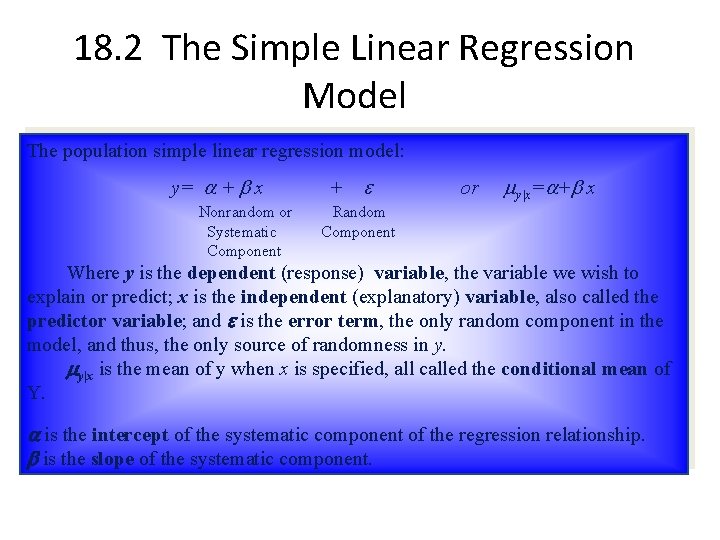
18. 2 The Simple Linear Regression Model The population simple linear regression model: y= a + x + or my|x=a+ x Nonrandom or Random Systematic Component Where y is the dependent (response) variable, the variable we wish to explain or predict; x is the independent (explanatory) variable, also called the predictor variable; and is the error term, the only random component in the model, and thus, the only source of randomness in y. my|x is the mean of y when x is specified, all called the conditional mean of Y. a is the intercept of the systematic component of the regression relationship. is the slope of the systematic component.

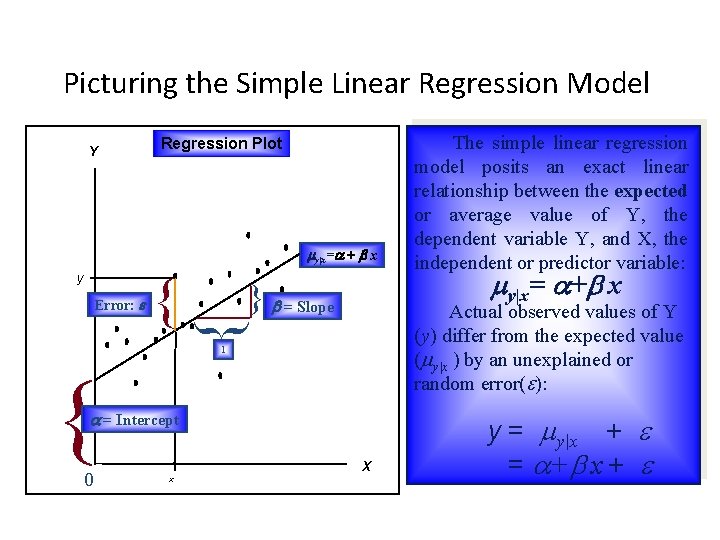
Picturing the Simple Linear Regression Model Y Regression Plot my|x=a + x y Error: } = Slope 1 { a = Intercept 0 X x my|x= a+ x Actual observed values of Y (y) differ from the expected value (my|x ) by an unexplained or random error( ): } { The simple linear regression model posits an exact linear relationship between the expected or average value of Y, the dependent variable Y, and X, the independent or predictor variable: y = my|x + = a+ x +

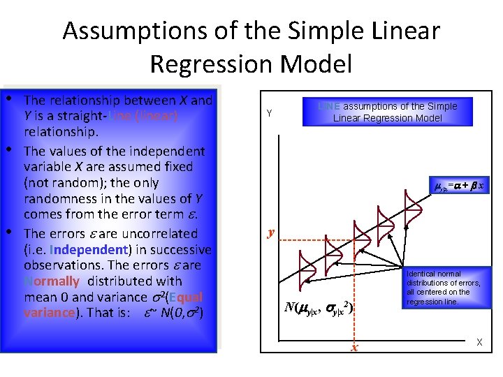
Assumptions of the Simple Linear Regression Model • • • The relationship between X and Y is a straight-Line (linear) relationship. The values of the independent variable X are assumed fixed (not random); the only randomness in the values of Y comes from the error term . The errors are uncorrelated (i. e. Independent) in successive observations. The errors are Normally distributed with mean 0 and variance 2(Equal variance). That is: ~ N(0, 2) Y LINE assumptions of the Simple Linear Regression Model my|x=a + x y N(my|x, sy|x 2) x Identical normal distributions of errors, all centered on the regression line. X

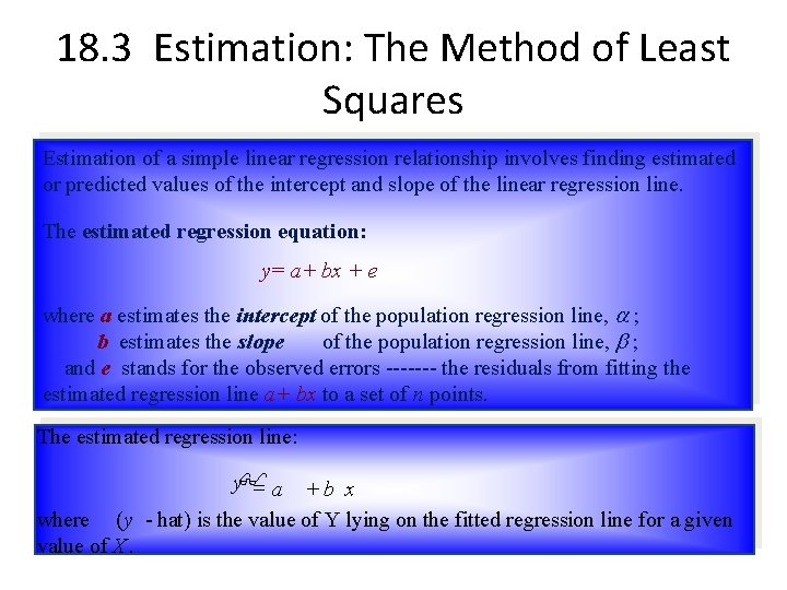
18. 3 Estimation: The Method of Least Squares Estimation of a simple linear regression relationship involves finding estimated or predicted values of the intercept and slope of the linear regression line. The estimated regression equation: y= a+ bx + e where a estimates the intercept of the population regression line, a ; b estimates the slope of the population regression line, ; and e stands for the observed errors ------- the residuals from fitting the estimated regression line a+ bx to a set of n points. The estimated regression line: = a +b x y$ where $ (y - hat) is the value of Y lying on the fitted regression line for a given value of X.

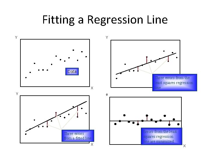
Fitting a Regression Line Y Y Data Three errors from the least squares regression line X X Y e Three errors from a fitted line X Errors from the least squares regression line are minimized X

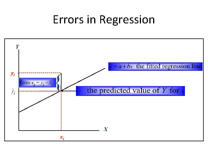
Errors in Regression Y yi . { X xi

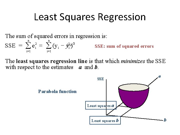
Least Squares Regression The sum of squared errors in regression is: n n 2 2 SSE = å e i = å (y i - y$ ) SSE: sum of squared errors i i=1 The least squares regression line is that which minimizes the SSE with respect to the estimates a and b. SSE a Parabola function Least squares a Least squares b b

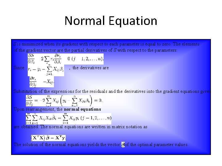
Normal Equation S is minimized when its gradient with respect to each parameter is equal to zero. The elements of the gradient vector are the partial derivatives of S with respect to the parameters: Since , the derivatives are Substitution of the expressions for the residuals and the derivatives into the gradient equations gives Upon rearrangement, the normal equations are obtained. The normal equations are written in matrix notation as The solution of the normal equations yields the vector of the optimal parameter values.

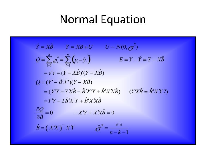
Normal Equation

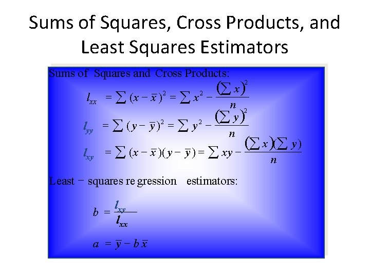
Sums of Squares, Cross Products, and Least Squares Estimators Sums of Squares and Cross Products: lxx = å ( x - x ) 2 = å x 2 lyy ( x) å - 2 n 2 ( y) å 2 2 = å (y - y ) = å y n lxy = å ( x - x )( y - y ) = å xy ( x )(å y ) å - Least - squares re gression estimators: lxy = b lxx a = y - b x n

Example

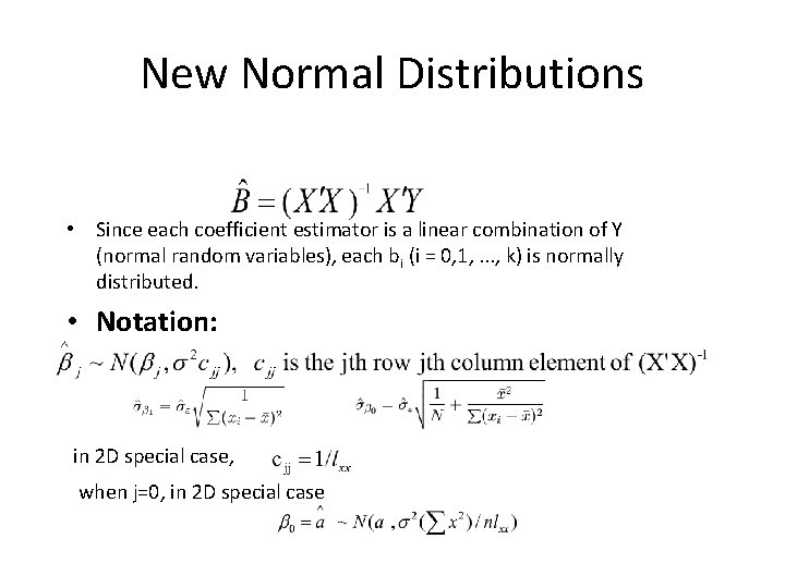
New Normal Distributions • Since each coefficient estimator is a linear combination of Y (normal random variables), each bi (i = 0, 1, . . . , k) is normally distributed. • Notation: in 2 D special case, when j=0, in 2 D special case

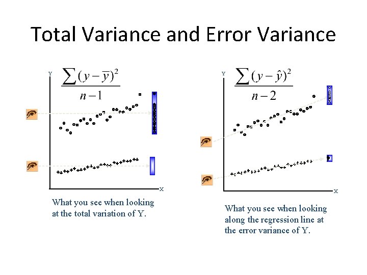
Total Variance and Error Variance Y Y X What you see when looking at the total variation of Y. X What you see when looking along the regression line at the error variance of Y.

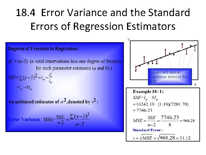
18. 4 Error Variance and the Standard Errors of Regression Estimators Y Square and sum all regression errors to find SSE. X

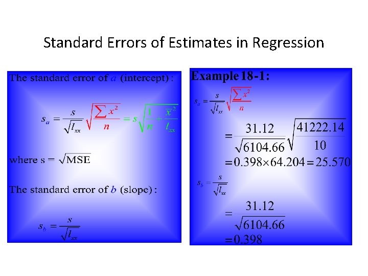
Standard Errors of Estimates in Regression

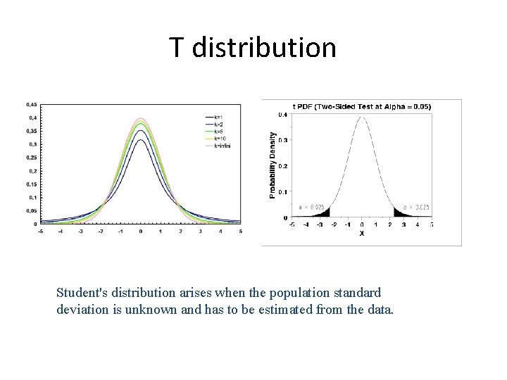
T distribution Student's distribution arises when the population standard deviation is unknown and has to be estimated from the data.

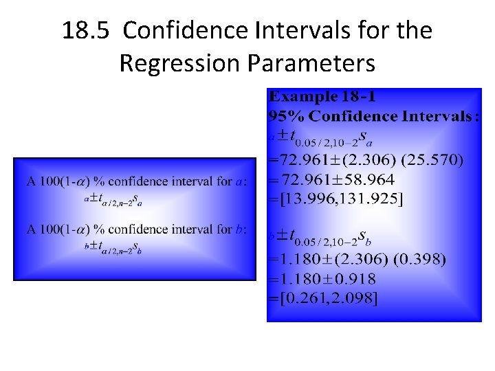
18. 5 Confidence Intervals for the Regression Parameters

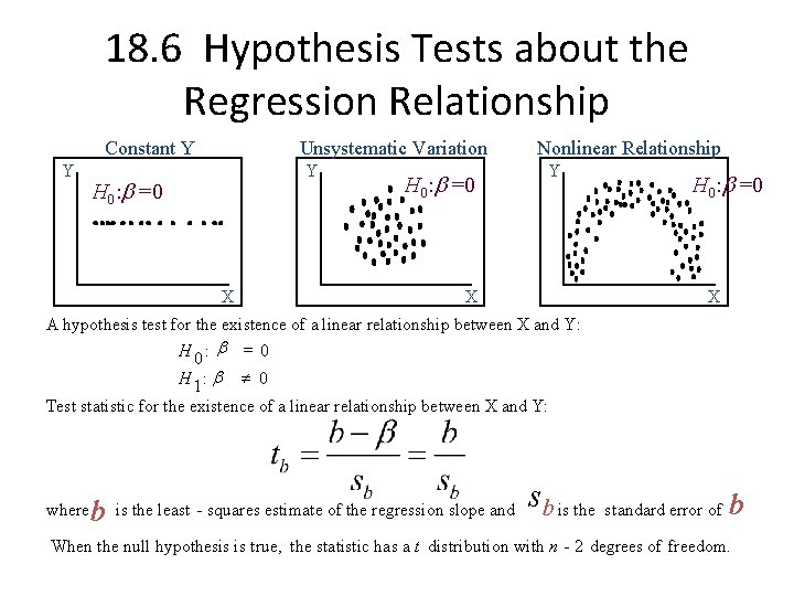
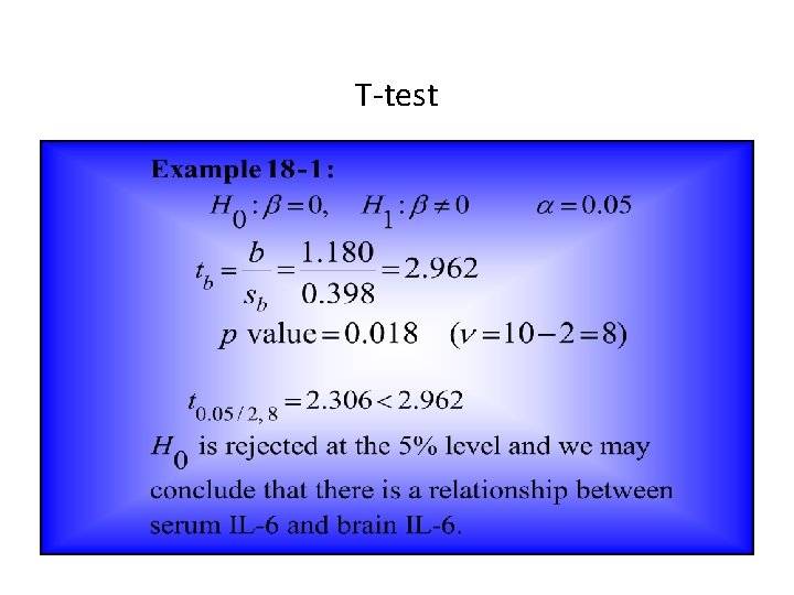
18. 6 Hypothesis Tests about the Regression Relationship Constant Y Y Unsystematic Variation Y H 0: =0 X H 0: =0 Nonlinear Relationship Y X H 0: =0 X A hypothesis test for the existence of a linear relationship between X and Y: H 0 : = 0 H 1 : ¹ 0 Test statistic for the existence of a linear relationship between X and Y: b is the least - squares estimate of the regression slope and sb is the standard error of b where When the null hypothesis is true, the statistic has a t distribution with n - 2 degrees of freedom.

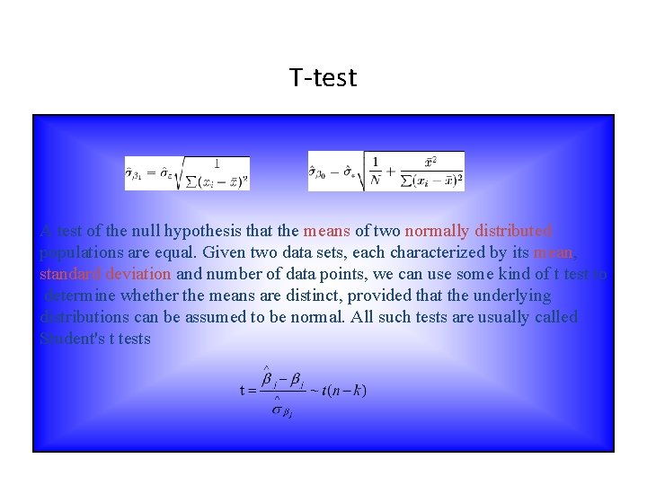
T-test A test of the null hypothesis that the means of two normally distributed populations are equal. Given two data sets, each characterized by its mean, standard deviation and number of data points, we can use some kind of t test to determine whether the means are distinct, provided that the underlying distributions can be assumed to be normal. All such tests are usually called Student's t tests

T-test

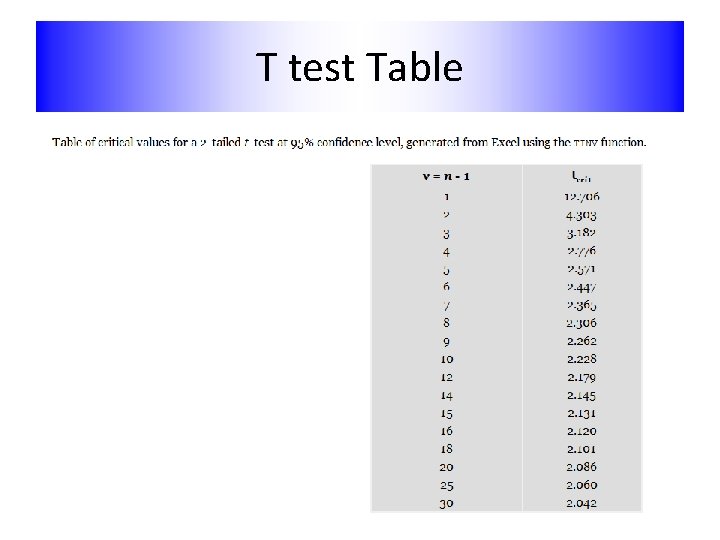
T test Table

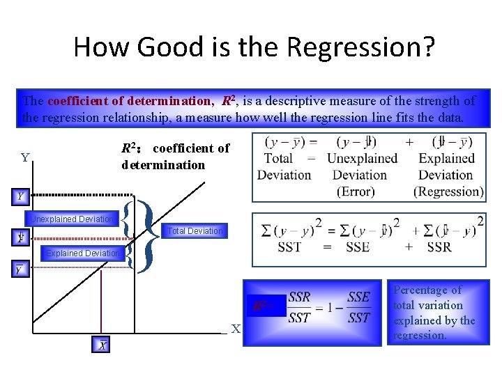
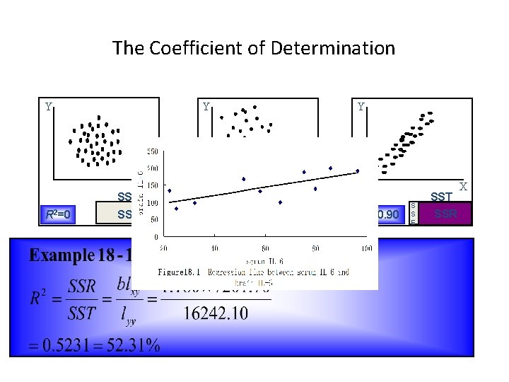
How Good is the Regression? The coefficient of determination, R 2, is a descriptive measure of the strength of the regression relationship, a measure how well the regression line fits the data. R 2： coefficient of determination Y . Unexplained Deviation } { Explained Deviation { Total Deviation R 2= X Percentage of total variation explained by the regression.

The Coefficient of Determination Y Y SST R 2=0 SSE X Y X R 2=0. 50 SST SSE SSR R 2=0. 90 S S E SST SSR X

Another Test • Earlier in this section you saw how to perform a t-test to compare a sample mean to an accepted value, or to compare two sample means. In this section, you will see how to use the F-test to compare two variances or standard deviations. • When using the F-test, you again require a hypothesis, but this time, it is to compare standard deviations. That is, you will test the null hypothesis H 0: σ12 = σ22 against an appropriate alternate hypothesis.

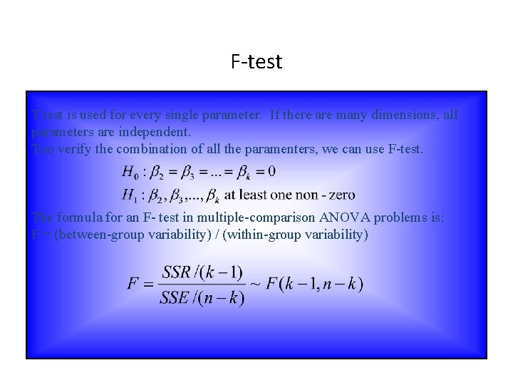
F-test T test is used for every single parameter. If there are many dimensions, all parameters are independent. Too verify the combination of all the paramenters, we can use F-test. The formula for an F- test in multiple-comparison ANOVA problems is: F = (between-group variability) / (within-group variability)

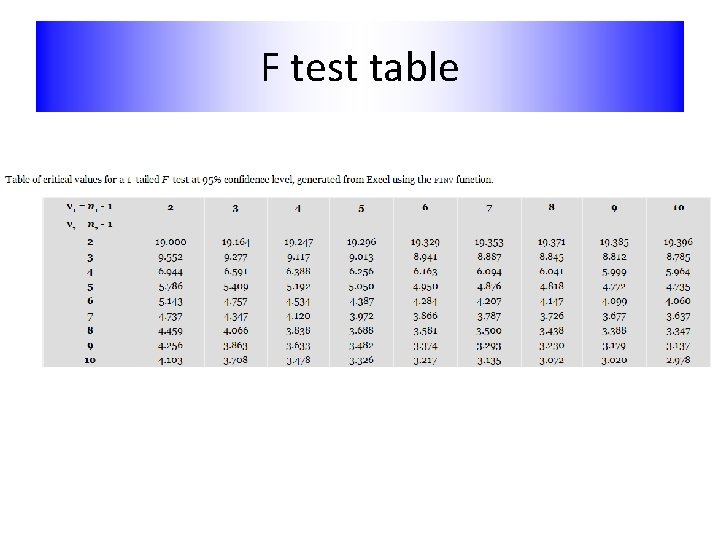
F test table

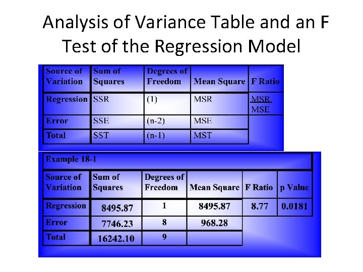
Analysis of Variance Table and an F Test of the Regression Model

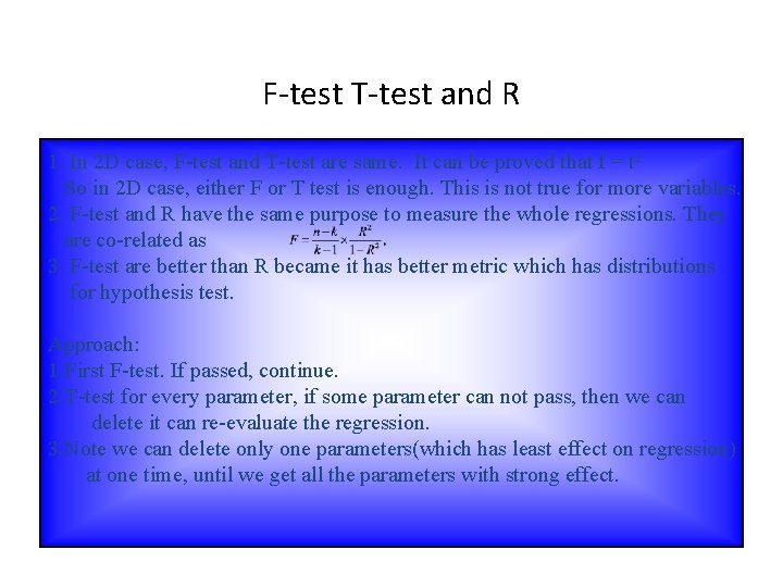
F-test T-test and R 1. In 2 D case, F-test and T-test are same. It can be proved that f = t 2 So in 2 D case, either F or T test is enough. This is not true for more variables. 2. F-test and R have the same purpose to measure the whole regressions. They are co-related as 3. F-test are better than R became it has better metric which has distributions for hypothesis test. Approach: 1. First F-test. If passed, continue. 2. T-test for every parameter, if some parameter can not pass, then we can delete it can re-evaluate the regression. 3. Note we can delete only one parameters(which has least effect on regression) at one time, until we get all the parameters with strong effect.

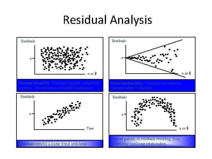
Residual Analysis Residuals 0 0 Homoscedasticity: Residuals appear completely random. No indication of model inadequacy. Residuals Heteroscedasticity: Variance of residuals changes when x changes. Residuals 0 0 Time Residuals exhibit a linear trend with time. Curved pattern in residuals resulting from underlying nonlinear relationship.

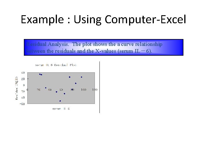
Example : Using Computer-Excel Residual Analysis. The plot shows the a curve relationship between the residuals and the X-values (serum IL－6).

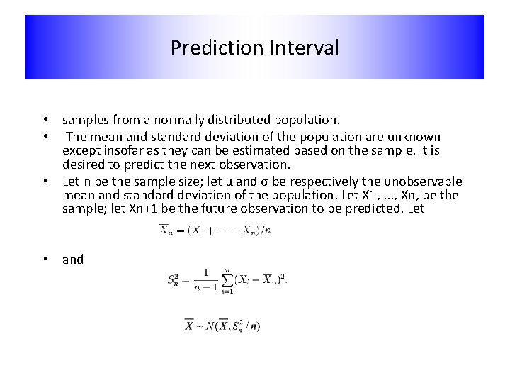
Prediction Interval • samples from a normally distributed population. • The mean and standard deviation of the population are unknown except insofar as they can be estimated based on the sample. It is desired to predict the next observation. • Let n be the sample size; let μ and σ be respectively the unobservable mean and standard deviation of the population. Let X 1, . . . , Xn, be the sample; let Xn+1 be the future observation to be predicted. Let • and

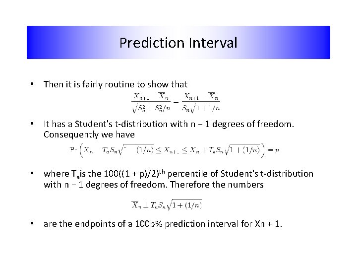
Prediction Interval • Then it is fairly routine to show that • It has a Student's t-distribution with n − 1 degrees of freedom. Consequently we have • where Tais the 100((1 + p)/2)th percentile of Student's t-distribution with n − 1 degrees of freedom. Therefore the numbers • are the endpoints of a 100 p% prediction interval for Xn + 1.

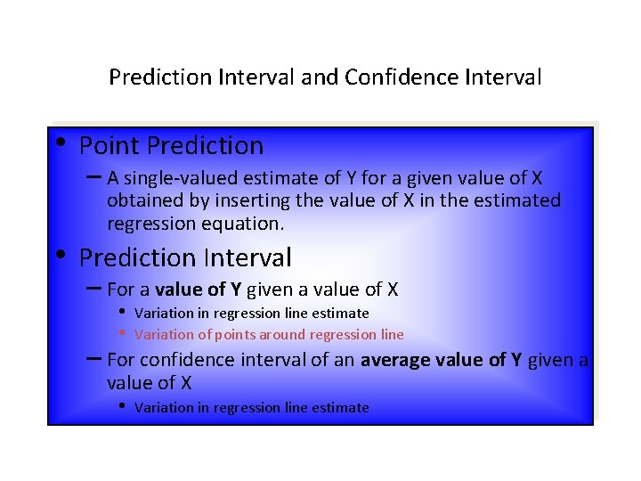
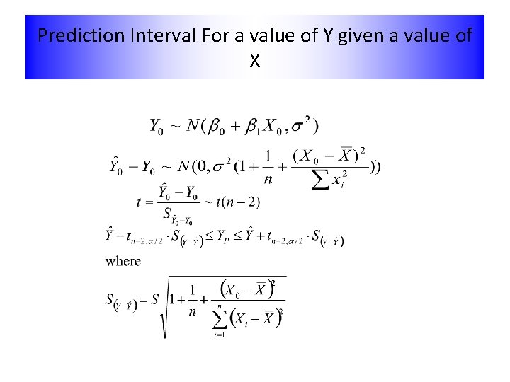
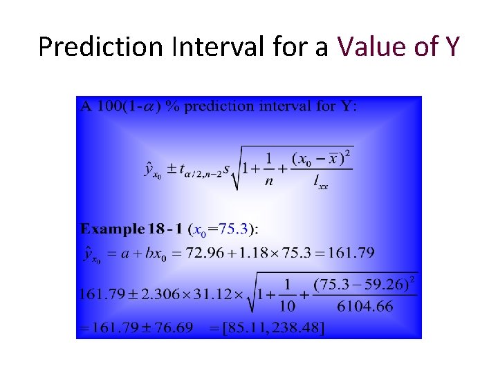
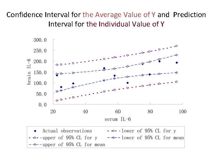
Prediction Interval and Confidence Interval • • Point Prediction – A single-valued estimate of Y for a given value of X obtained by inserting the value of X in the estimated regression equation. Prediction Interval – For a value of Y given a value of X • Variation in regression line estimate • Variation of points around regression line – For confidence interval of an average value of Y given a value of X • Variation in regression line estimate

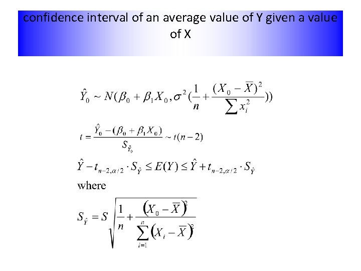
confidence interval of an average value of Y given a value of X

Confidence Interval for the Average Value of Y

Prediction Interval For a value of Y given a value of X

Prediction Interval for a Value of Y

Confidence Interval for the Average Value of Y and Prediction Interval for the Individual Value of Y

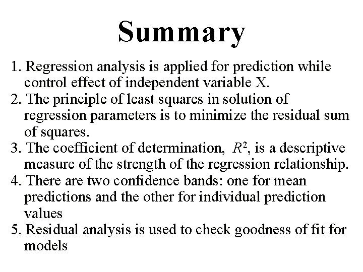
Summary 1. Regression analysis is applied for prediction while control effect of independent variable X. 2. The principle of least squares in solution of regression parameters is to minimize the residual sum of squares. 2, is a descriptive 3. The coefficient of determination, R 3. measure of the strength of the regression relationship. 4. There are two confidence bands: one for mean predictions and the other for individual prediction values 5. Residual analysis is used to check goodness of fit for models