Regression Analysis Scatter plots Regression analysis requires interval

Regression Analysis

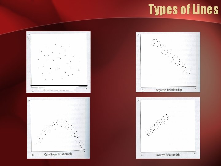
Scatter plots • Regression analysis requires interval and ratio-level data. • To see if your data fits the models of regression, it is wise to conduct a scatter plot analysis. • The reason? – Regression analysis assumes a linear relationship. If you have a curvilinear relationship or no relationship, regression analysis is of little use.

Types of Lines

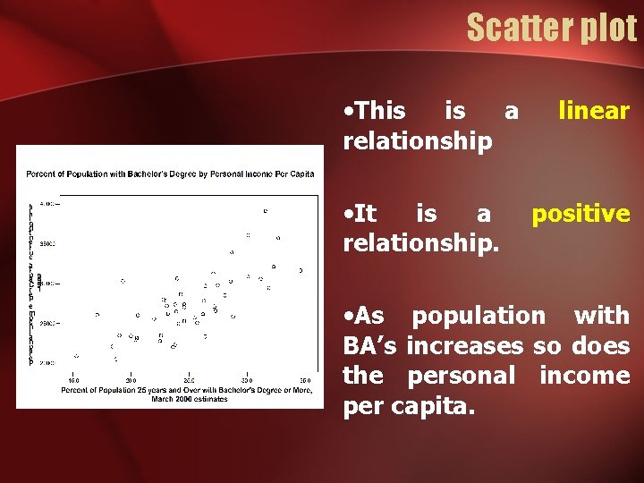
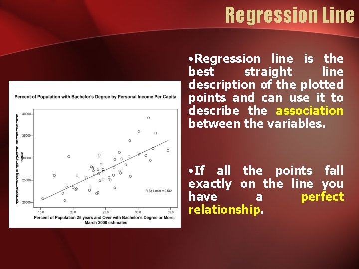
Scatter plot • This is a relationship • It is a relationship. linear positive • As population with BA’s increases so does the personal income per capita.

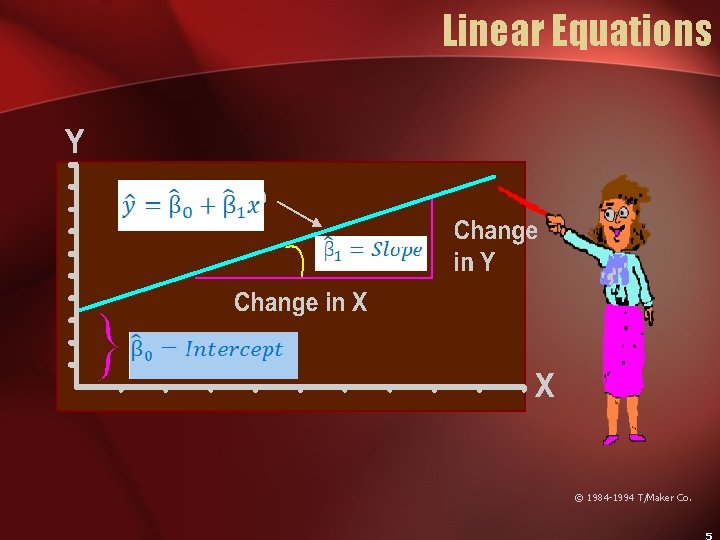
Linear Equations © 1984 -1994 T/Maker Co.

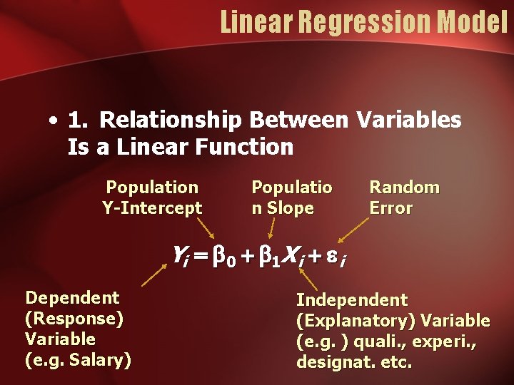
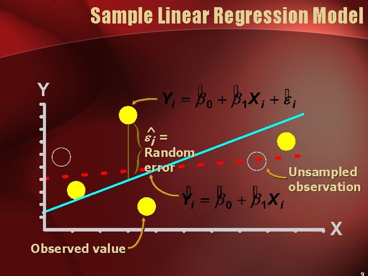
Linear Regression Model • 1. Relationship Between Variables Is a Linear Function Population Y-Intercept Populatio n Slope Random Error Yi 0 1 X i i Dependent (Response) Variable (e. g. Salary) Independent (Explanatory) Variable (e. g. ) quali. , experi. , designat. etc.

Regression Line • Regression line is the best straight line description of the plotted points and can use it to describe the association between the variables. • If all the points fall exactly on the line you have a perfect relationship.

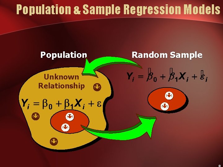
Population & Sample Regression Models Random Sample Population Unknown Relationship

Sample Linear Regression Model ^ i = Random error Observed value Unsampled observation

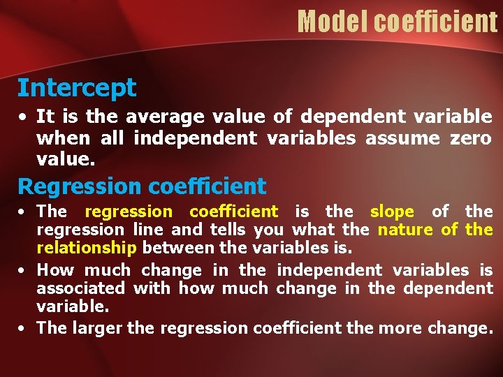
Model coefficient Intercept • It is the average value of dependent variable when all independent variables assume zero value. Regression coefficient • The regression coefficient is the slope of the regression line and tells you what the nature of the relationship between the variables is. • How much change in the independent variables is associated with how much change in the dependent variable. • The larger the regression coefficient the more change.

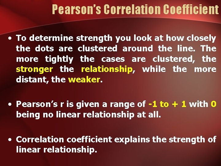
Pearson’s Correlation Coefficient • To determine strength you look at how closely the dots are clustered around the line. The more tightly the cases are clustered, the stronger the relationship, while the more distant, the weaker. • Pearson’s r is given a range of -1 to + 1 with 0 being no linear relationship at all. • Correlation coefficient explains the strength of linear relationship.

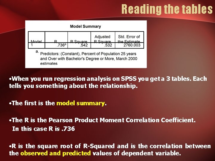
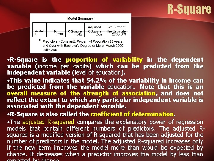
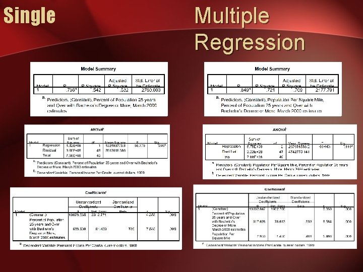
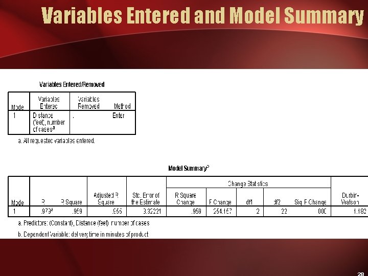
Reading the tables • When you run regression analysis on SPSS you get a 3 tables. Each tells you something about the relationship. • The first is the model summary. • The R is the Pearson Product Moment Correlation Coefficient. In this case R is. 736 • R is the square root of R-Squared and is the correlation between the observed and predicted values of dependent variable.

R-Square • R-Square is the proportion of variability in the dependent variable (income per capita) which can be predicted from the independent variable (level of education). • This value indicates that 54. 2% of the variability in income can be predicted from the variable education. Note that this is an overall measure of the strength of association, and does not reflect the extent to which any particular independent variable is associated with the dependent variable. • R-Square is also called the coefficient of determination. • The adjusted R-squared compares the explanatory power of regression models that contain different numbers of predictors. The adjusted Rsquared is a modified version of R-squared that has been adjusted for the number of predictors in the model. The adjusted R-squared increases only if the new term improves the model more than would be expected by chance. It decreases when a predictor improves the model by less than

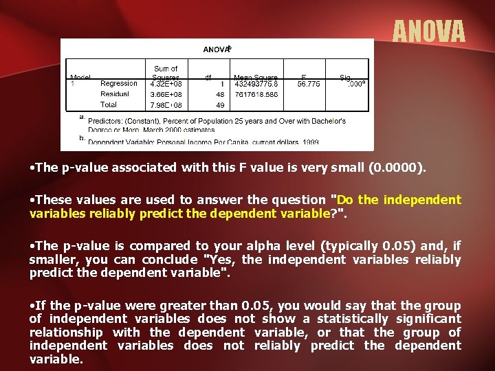
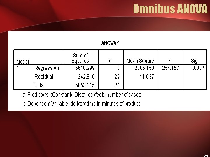
ANOVA • The p-value associated with this F value is very small (0. 0000). • These values are used to answer the question "Do the independent variables reliably predict the dependent variable? ". • The p-value is compared to your alpha level (typically 0. 05) and, if smaller, you can conclude "Yes, the independent variables reliably predict the dependent variable". • If the p-value were greater than 0. 05, you would say that the group of independent variables does not show a statistically significant relationship with the dependent variable, or that the group of independent variables does not reliably predict the dependent variable.

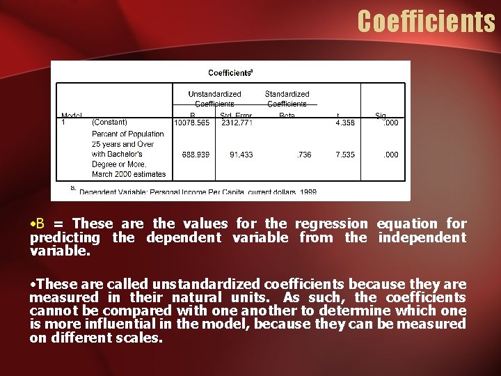
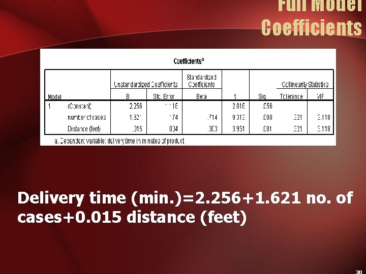
Coefficients • B = These are the values for the regression equation for predicting the dependent variable from the independent variable. • These are called unstandardized coefficients because they are measured in their natural units. As such, the coefficients cannot be compared with one another to determine which one is more influential in the model, because they can be measured on different scales.

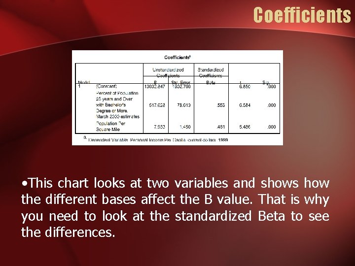
Coefficients • This chart looks at two variables and shows how the different bases affect the B value. That is why you need to look at the standardized Beta to see the differences.

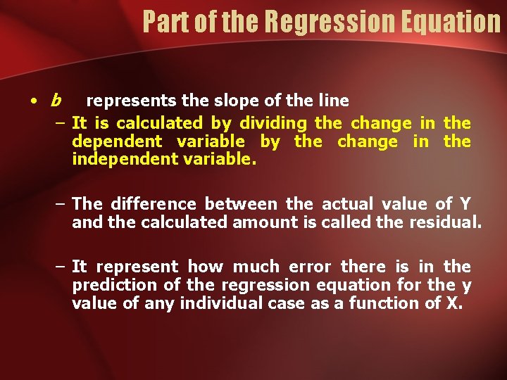
Part of the Regression Equation • b represents the slope of the line – It is calculated by dividing the change in the dependent variable by the change in the independent variable. – The difference between the actual value of Y and the calculated amount is called the residual. – It represent how much error there is in the prediction of the regression equation for the y value of any individual case as a function of X.

Single Multiple Regression

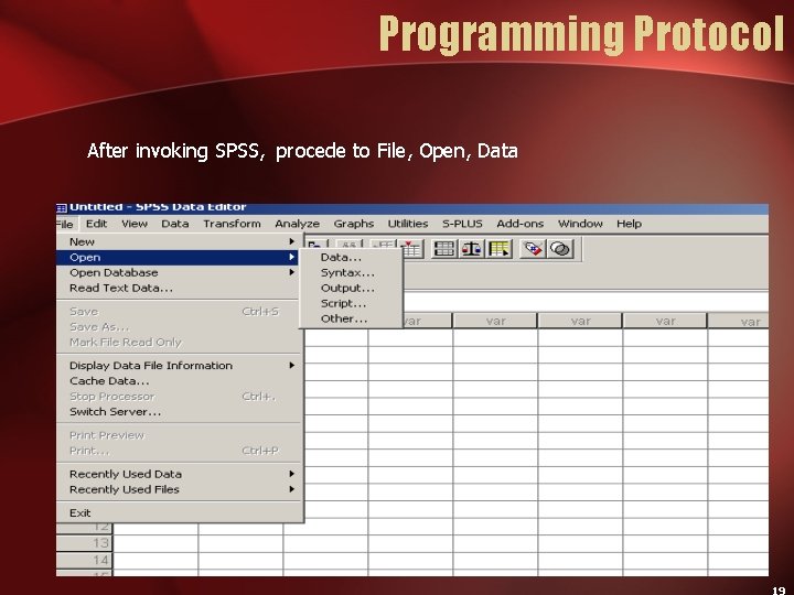
Programming Protocol After invoking SPSS, procede to File, Open, Data

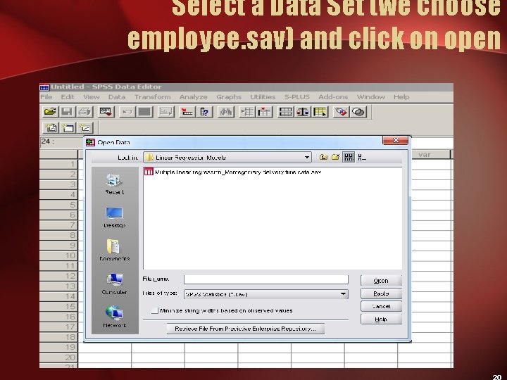
Select a Data Set (we choose employee. sav) and click on open

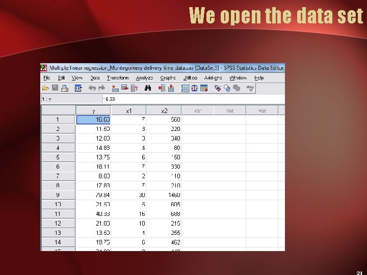
We open the data set

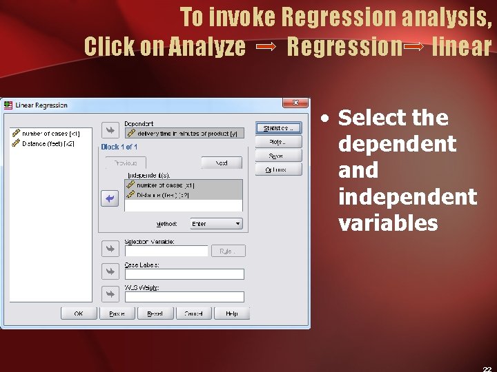
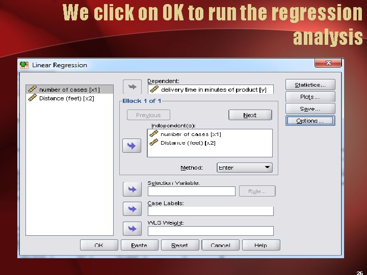
To invoke Regression analysis, Click on Analyze Regression linear • Select the dependent and independent variables

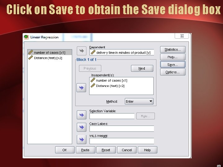
Analysis we wish • We are testing for effect of number of cases and distance in feet on delivery time (in minutes). • Objective is also to predict delivery time on the basis of number of cases and distance.

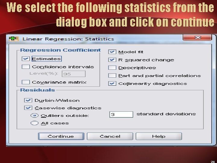
We select the following statistics from the dialog box and click on continue

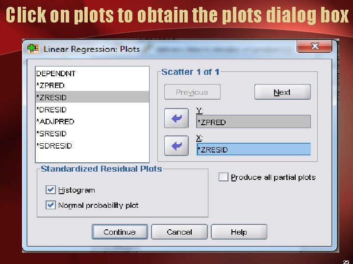
Click on plots to obtain the plots dialog box

We click on OK to run the regression analysis

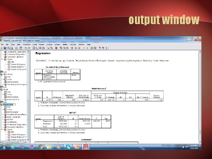
output window This shows that SPSS is reading the variables correctly 27

Variables Entered and Model Summary

Omnibus ANOVA Significance Tests for the Model at each stage of the analysis

Full Model Coefficients Delivery time (min. )=2. 256+1. 621 no. of cases+0. 015 distance (feet)

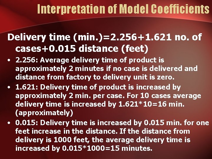
Interpretation of Model Coefficients Delivery time (min. )=2. 256+1. 621 no. of cases+0. 015 distance (feet) • 2. 256: Average delivery time of product is approximately 2 minutes if no case is delivered and distance from factory to delivery unit is zero. • 1. 621: Delivery time of product is increased by approximately 2 min. per case. For 10 cases average delivery time is increased by 1. 621*10=16 min. (approximately) • 0. 015: Delivery time is increased by 0. 015 min. for one feet increase in the distance. If the distance from delivery is 1000 feet, the average delivery time is increased by 0. 015*1000=15 minutes.

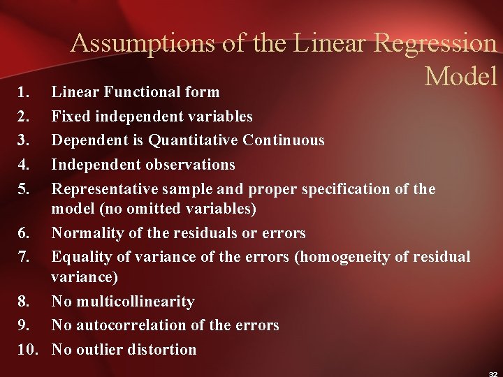
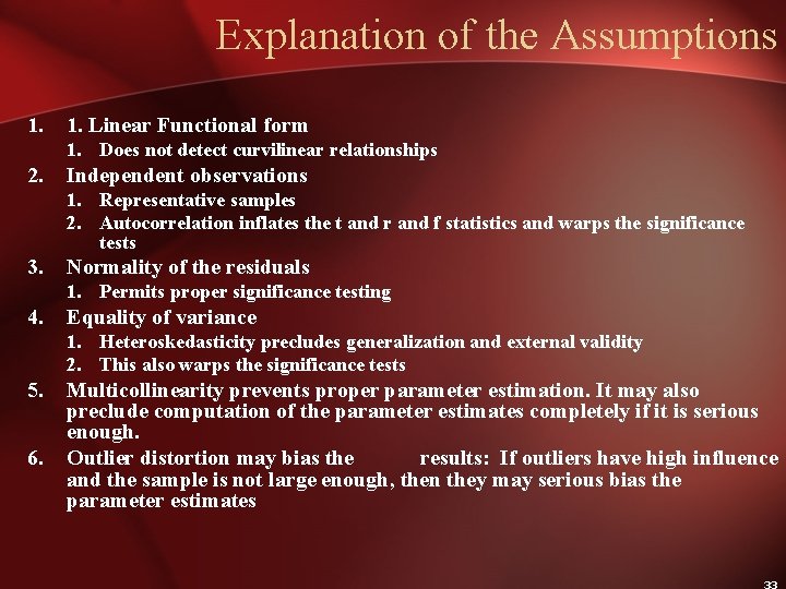
1. 2. 3. 4. 5. Assumptions of the Linear Regression Model Linear Functional form Fixed independent variables Dependent is Quantitative Continuous Independent observations Representative sample and proper specification of the model (no omitted variables) 6. Normality of the residuals or errors 7. Equality of variance of the errors (homogeneity of residual variance) 8. No multicollinearity 9. No autocorrelation of the errors 10. No outlier distortion

Explanation of the Assumptions 1. Linear Functional form 1. Does not detect curvilinear relationships 2. Independent observations 1. Representative samples 2. Autocorrelation inflates the t and r and f statistics and warps the significance tests 3. Normality of the residuals 1. Permits proper significance testing 4. Equality of variance 1. Heteroskedasticity precludes generalization and external validity 2. This also warps the significance tests 5. 6. Multicollinearity prevents proper parameter estimation. It may also preclude computation of the parameter estimates completely if it is serious enough. Outlier distortion may bias the results: If outliers have high influence and the sample is not large enough, then they may serious bias the parameter estimates

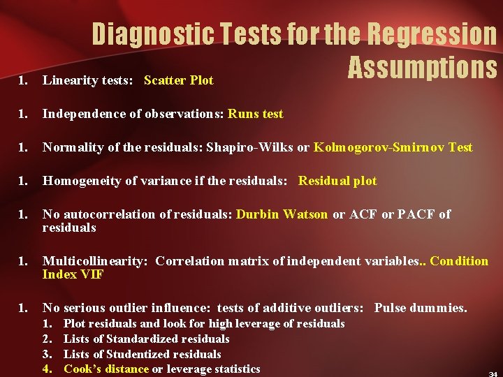
1. Diagnostic Tests for the Regression Assumptions Linearity tests: Scatter Plot 1. Independence of observations: Runs test 1. Normality of the residuals: Shapiro-Wilks or Kolmogorov-Smirnov Test 1. Homogeneity of variance if the residuals: Residual plot 1. No autocorrelation of residuals: Durbin Watson or ACF or PACF of residuals 1. Multicollinearity: Correlation matrix of independent variables. . Condition Index VIF 1. No serious outlier influence: tests of additive outliers: Pulse dummies. 1. 2. 3. 4. Plot residuals and look for high leverage of residuals Lists of Standardized residuals Lists of Studentized residuals Cook’s distance or leverage statistics

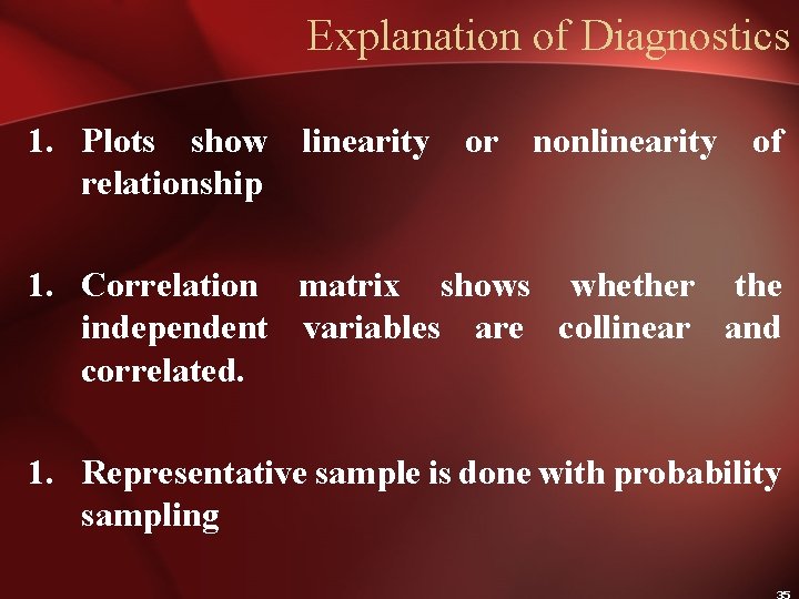
Explanation of Diagnostics 1. Plots show linearity or nonlinearity of relationship 1. Correlation matrix shows whether the independent variables are collinear and correlated. 1. Representative sample is done with probability sampling

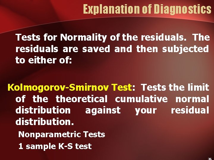
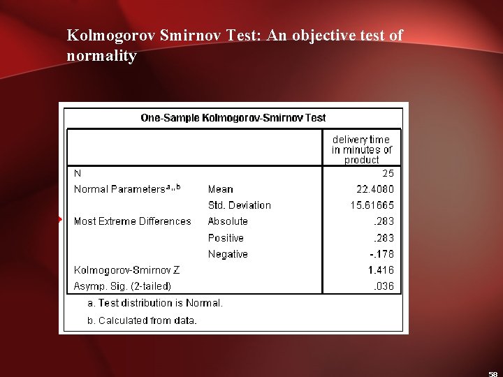
Explanation of Diagnostics Tests for Normality of the residuals. The residuals are saved and then subjected to either of: Kolmogorov-Smirnov Test: Tests the limit of theoretical cumulative normal distribution against your residual distribution. Nonparametric Tests 1 sample K-S test

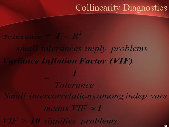
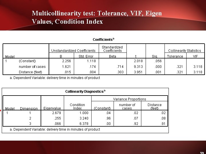
Collinearity Diagnostics

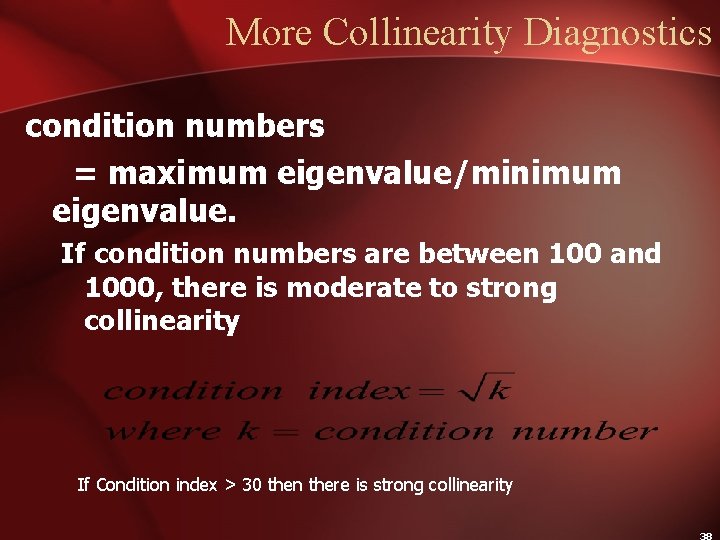
More Collinearity Diagnostics condition numbers = maximum eigenvalue/minimum eigenvalue. If condition numbers are between 100 and 1000, there is moderate to strong collinearity If Condition index > 30 then there is strong collinearity

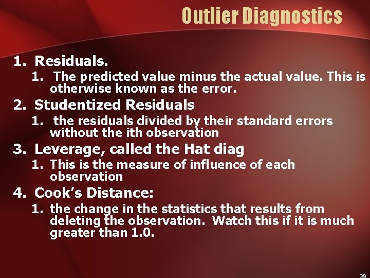
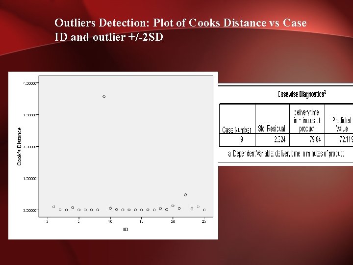
Outlier Diagnostics 1. Residuals. 1. The predicted value minus the actual value. This is otherwise known as the error. 2. Studentized Residuals 1. the residuals divided by their standard errors without the ith observation 3. Leverage, called the Hat diag 1. This is the measure of influence of each observation 4. Cook’s Distance: 1. the change in the statistics that results from deleting the observation. Watch this if it is much greater than 1. 0.

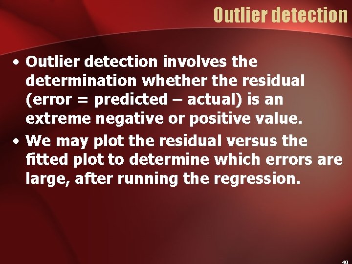
Outlier detection • Outlier detection involves the determination whether the residual (error = predicted – actual) is an extreme negative or positive value. • We may plot the residual versus the fitted plot to determine which errors are large, after running the regression.

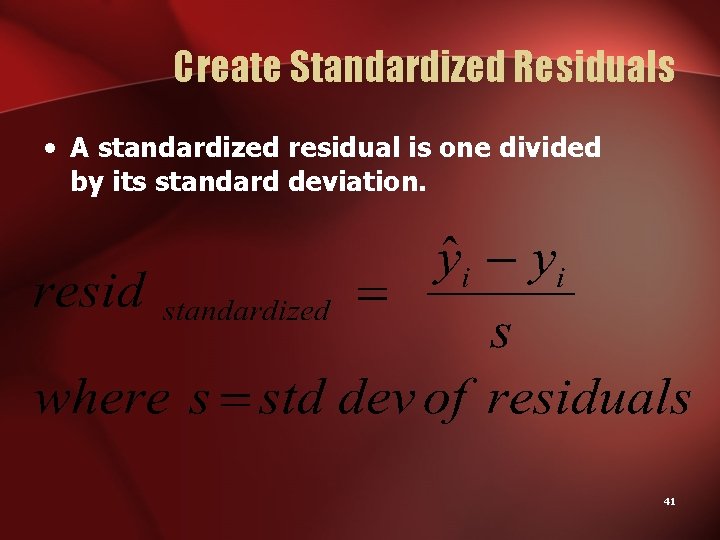
Create Standardized Residuals • A standardized residual is one divided by its standard deviation. 41

Limits of Standardized Residuals If the standardized residuals have values in excess of 3. 5 and -3. 5, they are outliers. If the absolute values are less than 3. 5, as these are, then there are no outliers While outliers by themselves only distort mean prediction when the sample size is small enough, it is important to gauge the influence of outliers.

Outlier Influence • Suppose we had a different data set with two outliers. • We tabulate the standardized residuals and obtain the following output:

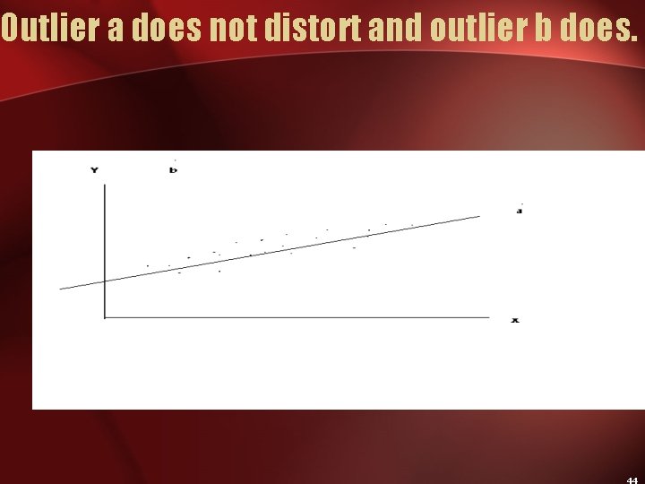
Outlier a does not distort and outlier b does.

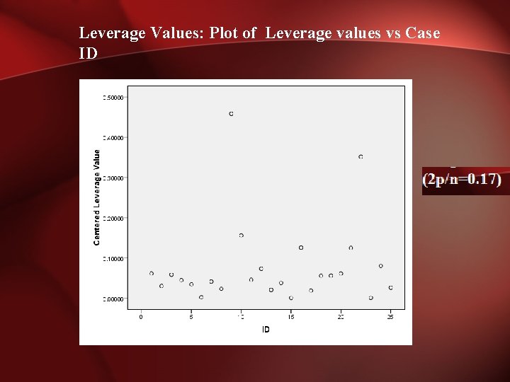
Leverage and the Hat matrix 1. 2. 3. 4. 5. 6. The hat matrix transforms Y into the predicted scores. The diagonals of the hat matrix indicate which values will be outliers or not. The diagonals are therefore measures of leverage. Leverage is bounded by two limits: 1/n and 1. The closer the leverage is to unity, the more leverage the value has. The trace of the hat matrix = the number of variables in the model. When the leverage > 2 p/n there is high leverage according to Belsley et al. (1980) cited in Long, J. F. Modern Methods of Data Analysis (p. 262). For smaller samples, Vellman and Welsch (1981) suggested that 3 p/n is the criterion.

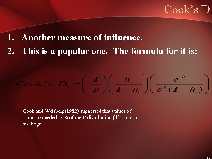
Cook’s D 1. Another measure of influence. 2. This is a popular one. The formula for it is: Cook and Weisberg(1982) suggested that values of D that exceeded 50% of the F distribution (df = p, n-p) are large.

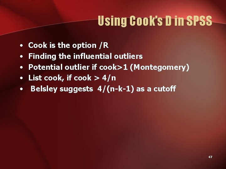
Using Cook’s D in SPSS • • • Cook is the option /R Finding the influential outliers Potential outlier if cook>1 (Montegomery) List cook, if cook > 4/n Belsley suggests 4/(n-k-1) as a cutoff 47

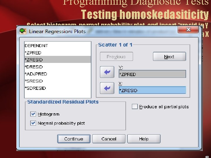
Programming Diagnostic Tests Testing homoskedasiticity Select histogram, normal probability plot, and insert *zresid in Y and *zpred in X Then click on continue

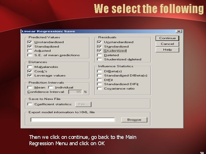
Click on Save to obtain the Save dialog box

We select the following Then we click on continue, go back to the Main Regression Menu and click on OK

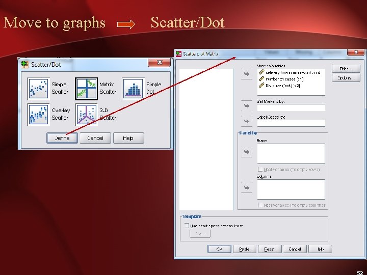
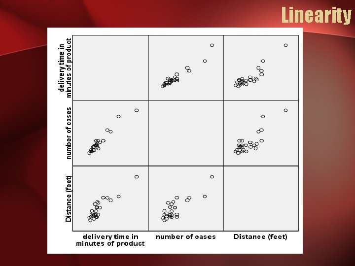
Check for linear Functional Form • Run a matrix plot of the dependent variable against each independent variable to be sure that the relationship is linear.

Move to graphs Scatter/Dot

Linearity

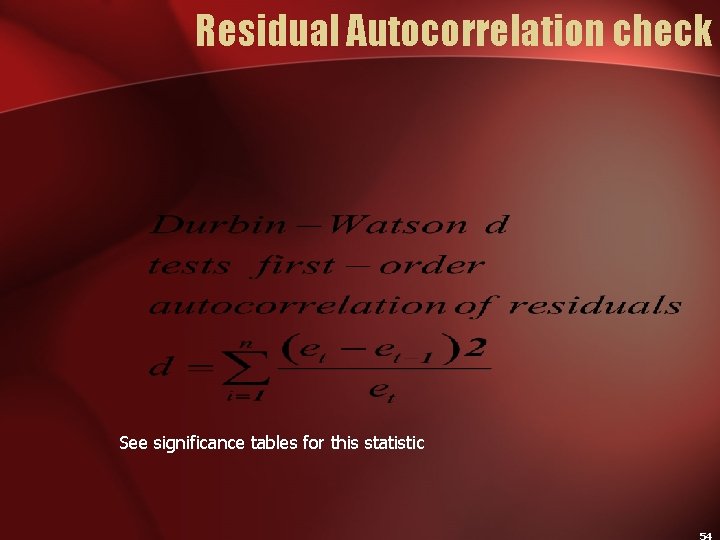
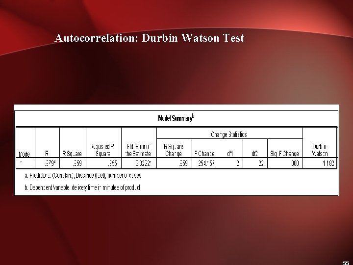
Residual Autocorrelation check See significance tables for this statistic

Autocorrelation: Durbin Watson Test

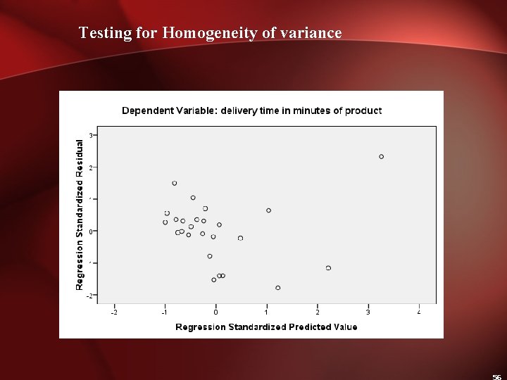
Testing for Homogeneity of variance

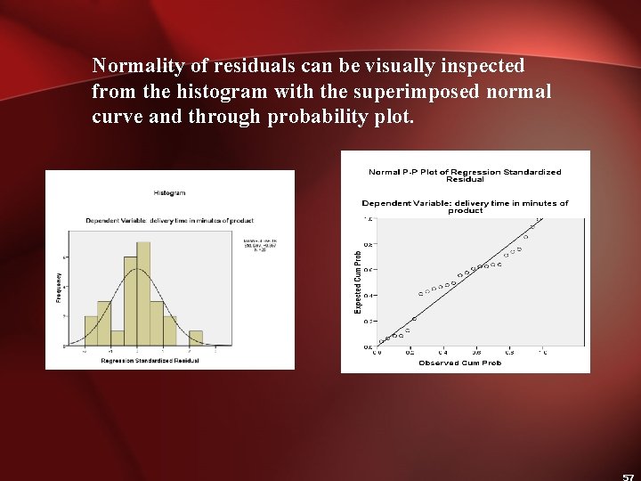
Normality of residuals can be visually inspected from the histogram with the superimposed normal curve and through probability plot.

Kolmogorov Smirnov Test: An objective test of normality

Multicollinearity test: Tolerance, VIF, Eigen Values, Condition Index

Outliers Detection: Plot of Cooks Distance vs Case ID and outlier +/-2 SD

Leverage Values: Plot of Leverage values vs Case ID

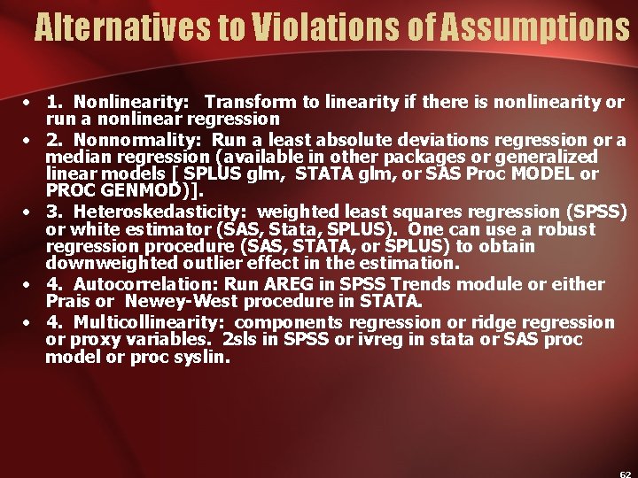
Alternatives to Violations of Assumptions • 1. Nonlinearity: Transform to linearity if there is nonlinearity or run a nonlinear regression • 2. Nonnormality: Run a least absolute deviations regression or a median regression (available in other packages or generalized linear models [ SPLUS glm, STATA glm, or SAS Proc MODEL or PROC GENMOD)]. • 3. Heteroskedasticity: weighted least squares regression (SPSS) or white estimator (SAS, Stata, SPLUS). One can use a robust regression procedure (SAS, STATA, or SPLUS) to obtain downweighted outlier effect in the estimation. • 4. Autocorrelation: Run AREG in SPSS Trends module or either Prais or Newey-West procedure in STATA. • 4. Multicollinearity: components regression or ridge regression or proxy variables. 2 sls in SPSS or ivreg in stata or SAS proc model or proc syslin.

Nonparametric Alternatives 1. If there is nonlinearity, transform to linearity first. 2. If there is heteroskedasticity, use robust standard errors with STATA or SAS or SPLUS. 3. If there is non-normality, use quantile regression with bootstrapped standard errors in STATA or SPLUS. 4. If there is autocorrelation of residuals, use Newey-West autoregression or First order autocorrelation correction with Areg. If there is higher order autocorrelation, use Box Jenkins ARIMA modeling.