Program Analysis and Verification 0368 4479 Noam Rinetzky

Program Analysis and Verification 0368 -4479 Noam Rinetzky Lecture 5: Abstract Interpretation Slides credit: Roman Manevich, Mooly Sagiv, Eran Yahav

Abstract Interpretation [Cousot’ 77] • Mathematical foundation of static analysis 2

Required knowledge ü Collecting semantics ü Abstract semantics (over lattices) ü Algorithm to compute abstract semantics (chaotic iteration) • Connection between collecting semantics and abstract semantics • Abstract transformers 3

Recap • We defined a reference semantics – the collecting semantics • We defined an abstract semantics for a given lattice and abstract transformers • We defined an algorithm to compute abstract least fixed-point when transformers are monotone and lattice obeys ACC • Questions: 1. What is the connection between the two least fixedpoints? 2. Transformer monotonicity is required for termination – what should we require for correctness? 4

Recap • We defined a reference semantics – the collecting semantics • We defined an abstract semantics for a given lattice and abstract transformers • We defined an algorithm to compute abstract least fixed-point when transformers are monotone and lattice obeys ACC • Questions: 1. What is the connection between the two least fixedpoints? 2. Transformer monotonicity is required for termination – what should we require for correctness? 5

Galois Connection • Given two complete lattices C, � C) C = (DC, � – concrete domain A, � A) – abstract domain A = (DA, � • A Galois Connection (GC) is quadruple (C, , , A) that relates C and A via the monotone functions – The abstraction function : DC DA – The concretization function : DA DC • for every concrete element c DC and abstract element a DA ( (a)) a and c ( (c)) • Alternatively (c) �a iff c � (a) 6

Galois Connection: c ( (c)) C A The most precise (least) element in A representing c � ( (c)) 3 c 1 2 (c) 7

Galois Connection: ( (a)) a C What a represents in C (its meaning) A (a) 2 a � 1 ( (a)) 3 8

Example: lattice of equalities • Concrete lattice: C = (2 State, � , � , State) • Abstract lattice: EQ = { x=y | x, y Var} A = (2 EQ, � , � , EQ , � ) – Treat elements of A as both formulas and sets of constraints • Useful for copy propagation – a compiler optimization • (X) = ? (Y) = ? 9

Example: lattice of equalities • Concrete lattice: C = (2 State, � , � , State) • Abstract lattice: EQ = { x=y | x, y Var} A = (2 EQ, � , � , EQ , � ) – Treat elements of A as both formulas and sets of constraints • Useful for copy propagation – a compiler optimization • (s) = ({s}) = { x=y | s x = s y} that is s �x=y A { (s) | s X} (X) = � { (s) | s X} = � (Y) = { s | s �� Y } = models(� Y) 10

Galois Connection: c ( (c)) C x=x, y=y, z=z � 3 1 [x� 5, y� 5, z� 5] 4 � … [x� 6, y� 6, z� 6] [x� 5, y� 5, z� 5] [x� 4, y� 4, z� 4] … A x=x, y=y, z=z, x=y, y=x, 2 x=z, z=x, y=z, z=y The most precise (least) element in A representing [x� 5, y� 5, z� 5] 11

Most precise abstract representation (c) = � {c’ | c � (c’)} C A 6 � � 5 7 3 9 c 4 2 � 8 (c) 1 12

Most precise abstract representation (c) = � {c’ | c � (c’)} C A x=y � � 5 7 3 9 c 1 [x� 5, y� 5, z� 5] 6 x=y, z=y 4 2 x=y, y=z (c)= 8 x=x, y=y, z=z, x=y, y=x, x=z, z=x, y=z, z=y 13

Galois Connection: ( (a)) a C … [x� 6, y� 6, z� 6] [x� 5, y� 5, z� 5] [x� 4, y� 4, z� 4] … What a represents in C (its meaning) A 1 2 � x=y, y=z � is called a semantic reduction 3 x=x, y=y, z=z, x=y, y=x, x=z, z=x, y=z, z=y 14

Galois Insertion � a: ( (a))=a C How can we obtain a Galois Insertion from a Galois Connection? … [x� 6, y� 6, z� 6] [x� 5, y� 5, z� 5] [x� 4, y� 4, z� 4] … 2 A All elements are reduced 1 x=x, y=y, z=z, x=y, y=x, x=z, z=x, y=z, z=y 15

Properties of a Galois Connection • The abstraction and concretization functions uniquely determine each other: (a) = � {c | (c) �a} (c) = � {a | c � (a)} 16

Abstracting (disjunctive) sets • It is usually convenient to first define the abstraction of single elements (s) = ({s}) • Then lift the abstraction to sets of elements A { (s) | s X} (X) = � 17

The case of symbolic domains • An important class of abstract domains are symbolic domains – domains of formulas • C = (2 State, � , � , State) A, � A) A = (DA, � • If DA is a set of formulas then the abstraction of a state is defined as A{ | s � (s) = ({s}) = � } the least formula from DA that s satisfies • The abstraction of a set of states is A { (s) | s X} (X) = � • The concretization is ( ) = { s | s � } = models( ) 18

Inducing along the connections • Assume the complete lattices C, � C) C = (DC, � A, � A) A = (DA, � M, � M) M = (DM, � and Galois connections GCC, A=(C, C, A, C, A) and GCA, M=(A, A, M, A, M) • Lemma: both connections induce the GCC, M= (C, C, M, C, M) defined by C, M = C, A � A, M and M, C = M, A � A, C 19

Inducing along the connections C A A, C c’ 5 c 1 M M, A 4 C, A 2 C, A(c) A, M 3 a’ = A, M( C, A(c)) 20

Sound abstract transformer • Given two lattices C, � C) C = (DC, � A, � A) A = (DA, � and GCC, A=(C, , , A) with • A concrete transformer f : DC DC an abstract transformer f# : DA DA • We say that f# is a sound transformer (w. r. t. f) if • � c: f(c)=c’ (f#(c)) � (c’) • For every a and a’ such that A f#(a) (f( (a))) � 21

Transformer soundness condition 1 � c: f(c)=c’ (f#(c)) � (c’) A � C 5 1 f 2 3 f# 4 22

Transformer soundness condition 2 � a: f#(a)=a’ f( (a)) � (a’) C A f 3 � 4 5 1 f# 2 23

Best (induced) transformer f#(a)= (f( (a))) C f A 4 3 1 2 Problem: incomputable directly f# 24

Best abstract transformer [CC’ 77] • Best in terms of precision – Most precise abstract transformer – May be too expensive to compute • Constructively defined as f# = �f � – Induced by the GC • Not directly computable because first step is concretization • We often compromise for a “good enough” transformer – Useful tool: partial concretization 25

Transformer example • C = (2 State, � , � , State) • EQ = { x=y | x, y Var} A = (2 EQ, � , � , EQ , � ) • (s) = ({s}) = { x=y | s x = s y} that is s �x=y A { (s) | s X} (X) = � { (s) | s X} = � ( ) = { s | s � } = models( ) • Concrete: � x: =y�X = { s[x� s y] | s X} #X=? • Abstract: � x: =y� 26

Developing a transformer for EQ - 1 • Input has the form X = � {a=b} • sp(x: =expr, � � )=� v. x=expr[v/x] �� [v/x] • sp(x: =y, � X) = � v. x=y[v/x] �� {a=b}[v/x] = … • Let’s define helper notations: – EQ(X, y) = {y=a, b=y �X} • Subset of equalities containing y – EQc(X, y) = X EQ(X, y) • Subset of equalities not containing y 27

Developing a transformer for EQ - 2 • sp(x: =y, � X) = � v. x=y[v/x] �� {a=b}[v/x] = … • Two cases – x is y: sp(x: =y, � X) = X – x is different from y: sp(x: =y, � X) = � v. x=y � EQ(X, x)[v/x] �EQc(X, x)[v/x] = x=y �EQc(X, x) �� v. EQ(X, x)[v/x] �x=y �EQc(X, x) #1 X = x=y � • Vanilla transformer: � x: =y� EQc(X, x) #1 � • Example: � x: =y� {x=p, q=x, m=n} = � {x=y, m=n} Is this the most precise result? 28

Developing a transformer for EQ - 3 #1 � • � x: =y� {x=p, x=q, m=n} = � {x=y, m=n} �� {x=y, m=n, p=q} – Where does the information p=q come from? • sp(x: =y, � X) = x=y �EQc(X, x) �� v. EQ(X, x)[v/x] • � v. EQ(X, x)[v/x] holds possible equalities between different a’s and b’s – how can we account for that? 29

Developing a transformer for EQ - 4 • Define a reduction operator: Explicate(X) = if exist {a=b, b=c}� X but not {a=c} � X then Explicate(X� {a=c}) else X #2 = � #1 � • Define � x: =y� Explicate #2(� • � x: =y� {x=p, x=q, m=n}) = � {x=y, m=n, p=q} is the best transformer? 30

Developing a transformer for EQ - 5 #2 (� • � x: =y� {y=z}) = {x=y, y=z} �{x=y, y=z, x=z} • Idea: apply reduction operator again after the vanilla transformer #3 = Explicate � #1 � • � x: =y� Explicate • Observation : after the first time we apply Explicate, all subsequent values will be in the image of the abstraction so really we only need to apply it once to the input #(X) = Explicate � #1 • Finally: � x: =y� – Best transformer for reduced elements (elements in the image of the abstraction) 31

Negative property of best transformers • Let f# = �f � • Best transformer does not compose (f(f( (a)))) f#(f#(a)) 32

(f(f( (a)))) f#(f#(a)) C A 9 4 2 f f � 7 f f# 5 8 3 6 1 f# 33

Soundness theorem 1 1. Given two complete lattices C, � C) C = (DC, � A, � A) A = (DA, � and GCC, A=(C, , , A) with 2. Monotone concrete transformer f : DC DC 3. Monotone abstract transformer f# : DA DA 4. a DA : f( (a)) (f#(a)) Then lfp(f) (lfp(f#)) (lfp(f)) lfp(f#) 34

Soundness theorem 1 a DA : f( (a)) (f#(a)) � a DA : fn( (a)) (f#n(a)) � a DA : lfp(fn)( (a)) (lfp(f#n)(a)) �lfp(f) � lfp(f#) � C A lpf(f) � lpf(f#) � fn � f#n � … … f 2 � f#3� f#2 � f� f# � f 3 � � � 35

Soundness theorem 2 1. Given two complete lattices C, � C) C = (DC, � A, � A) A = (DA, � and GCC, A=(C, , , A) with 2. Monotone concrete transformer f : DC DC 3. Monotone abstract transformer f# : DA DA 4. c DC : (f(c)) f#( (c)) Then (lfp(f)) lfp(f#) lfp(f) (lfp(f#)) 36

Soundness theorem 2 c DC : (f(c)) f#( (c)) � c DC : (fn(c)) f#n( (c)) � c DC : (lfp(f)(c)) lfp(f#)( (c)) �lfp(f) � lfp(f#) � C A lpf(f) � fn � f� � f#n � … … f 3 � f 2 � lpf(f#) � f#3� f#2 � f# � � 37

A recipe for a sound static analysis • Define an “appropriate” operational semantics • Define “collecting” structural operational semantics • Establish a Galois connection between collecting states and abstract states • Local correctness: show that the abstract interpretation of every atomic statement is sound w. r. t. the collecting semantics • Global correctness: conclude that the analysis is sound 38

Completeness • Local property: – forward complete: � c: (f#(c)) = (f(c)) – backward complete: � a: f( (a)) = (f#(a)) • A property of domain and the (best) transformer • Global property: – (lfp(f)) = lfp(f#) – lfp(f) = (lfp(f#)) • Very ideal but usually not possible unless we change the program model (apply strong abstraction) and/or aim for very simple properties 39

Forward complete transformer � c: (f#(c)) = (f(c)) C 1 f A 2 4 3 f# 40

Backward complete transformer � a: f( (a)) = (f#(a)) C f 3 A 5 1 f# 2 41

Global (backward) completeness � a: f( (a)) = (f#(a)) C �� a: fn( (a)) = (f#n(a)) � a DA : lfp(fn)( (a)) = (lfp(f#n)(a)) �lfp(f) �= lfp(f#) � A lpf(f) � lpf(f#) � fn � f#n � … … f 2 � f#3� f#2 � f� f# � f 3 � � � 42

Global (forward) completeness c DC : (f(c)) = f#( (c)) � c DC : (fn(c)) = f#n( (c)) � c DC : (lfp(f)(c)) = lfp(f#)( (c)) �lfp(f) �= lfp(f#) � C A lpf(f) � … f 3 � f 2 � f� � f#n � … fn � lpf(f#) � f#3� f#2 � f# � � 43

Example: Pointer Analysis

Plan • Understand the problem • Mention some applications • Simplified problem – Only variables (no object allocation) • • Reference analysis Andersen’s analysis Steensgaard’s analysis Generalize to handle object allocation 45

Constant propagation example x = 3; y = 4; z = x + 5; 46

Constant propagation example with pointers x = 3; Is x always 3 here? *p = 4; z = x + 5; 47

Constant propagation example with pointers p = &y; x = 3; *p = 4; z = x + x is always pointers affect if (? ) p = &x; most program analyses p = &x; x = 3; else *p = 4; p = &y; 5; z = x + 5; x = 3; *p = 4; z = x + 5; 3 x is always 4 x may be 3 or 4 (i. e. , x is unknown in our lattice) 48

Constant propagation example with pointers p = &y; x = 3; *p = 4; z = x + 5; p always points-to y if (? ) p = &x; else p = &y; x = 3; *p = 4; z = x + 5; p = &x; x = 3; *p = 4; z = x + 5; p always points-to x p may point-to x or y 49

Points-to Analysis • Determine the set of targets a pointer variable could point-to (at different points in the program) – “p points-to x” • “p stores the value &x” • “*p denotes the location x” – targets could be variables or locations in the heap (dynamic memory allocation) • p = &x; • p = new Foo(); or p = malloc (…); – must-point-to vs. may-point-to 50

Constant propagation example with pointers Can *p denote the same location as *q? *q = 3; *p = 4; z = *q + 5; what values can this take? 51

More terminology • *p and *q are said to be aliases (in a given concrete state) if they represent the same location • Alias analysis – Determine if a given pair of references could be aliases at a given program point – *p may-alias *q – *p must-alias *q 52

Pointer Analysis • Points-To Analysis – may-point-to – must-point-to • Alias Analysis – may-alias – must-alias 53

Applications • Compiler optimizations – Method de-virtualization – Call graph construction – Allocating objects on stack via escape analysis • Verification & Bug Finding – Datarace detection – Use in preliminary phases – Use in verification itself 54

Points-to analysis: a simple example p = &x; q = &y; if (? ) { q = p; } x = &a; y = &b; z = *q; {p=&x} {p=&x �q=&y} {p=&x {p=&x We will usually drop variable-equality information �q=&x} �(q=&y �q=&x) �x=&a} �(q=&y �q=&x) �x=&a �y=&b} �(q=&y� q=&x) �x=&a �y=&b �(z=x� z=y)} How would you construct an abstract domain to represent these abstract states? 55

Points-to lattice • Points-to – PT-factoids[x] = { x=&y | y Var} �false PT[x] = (2 PT-factoids, , �, false, PT-factoids[x]) (interpreted disjunctively) • How should combine them to get the abstract states in the example? {p=&x �(q=&y� q=&x) �x=&a �y=&b} 56

Points-to lattice • Points-to – PT-factoids[x] = { x=&y | y Var} �false PT[x] = (2 PT-factoids, , �, false, PT-factoids[x]) (interpreted disjunctively) • How should combine them to get the abstract states in the example? {p=&x �(q=&y� q=&x) �x=&a �y=&b} • D[x] = Disj(VE[x]) �Disj(PT[x]) • For all program variables: D = D[x 1] �… �D[xk] 57

Points-to analysis a = &y x = &a; y = &b; if (? ) { p = &x; } else { p = &y; } *x = &c; *p = &c; How should we handle this statement? Strong update {x=&a �y=&b �(p=&x� p=&y) �a=&y} {x=&a �y=&b �(p=&x� p=&y) �a=&c} {(x=&a� x=&c) �(y=&b� y=&c) �(p=&x� p=&y) �a=&c} Weak update 58

Questions • When is it correct to use a strong update? A weak update? • Is this points-to analysis precise? • What does it mean to say – p must-point-to x at program point u – p may-point-to x at program point u – p must-not-point-to x at program point u – p may-not-point-to x at program point u 59

Points-to analysis, formally • We must formally define what we want to compute before we can answer many such questions 60

PWhile syntax • A primitive statement is of the form • x : = null Omitted (for now) • x : = y • Dynamic memory allocation • x : = *y • Pointer arithmetic • Structures and fields • x : = &y; • Procedures • *x : = y • skip (where x and y are variables in Var) 61

PWhile operational semantics • • • State : (Var Z) �(Var Var� {null}) �x = y �s = �x = *y �s = �*x = y �s = �x = null �s = �x = &y �s = 62

PWhile operational semantics • • • State : (Var Z) �(Var Var� {null}) �x = y �s = s[x� s(y)] �x = *y �s = s[x� s(s(y))] must say what happens if null is �*x = y �s = s[s(x)� s(y)] dereferenced �x = null �s = s[x� null] �x = &y �s = s[x� y] 63

PWhile collecting semantics • CS[u] = set of concrete states that can reach program point u (CFG node) 64

Ideal PT Analysis: formal definition • Let u denote a node in the CFG • Define Ideal. Must. PT(u) to be { (p, x) | forall s in CS[u]. s(p) = x } • Define Ideal. May. PT(u) to be { (p, x) | exists s in CS[u]. s(p) = x } 65

May-point-to analysis: formal Requirement specification May/Must Point-To Analysis may Compute R: V -> 2 Vars’ such that R(u)⊇Ideal. May. PT(u) must For every vertex u in the CFG, compute a set R(u) such that R(u) ⊆ { (p, x) | " sÎCS[u]. s(p) = x } Var’ = Var U {null} 66

May-point-to analysis: formal Requirement specification Compute R: V -> 2 Vars’ such that R(u) ⊇ Ideal. May. PT(u) • An algorithm is said to be correct if the solution R it computes satisfies "uÎV. R(u) ⊇ Ideal. May. PT(u) • An algorithm is said to be precise if the solution R it computes satisfies "uÎV. R(u) = Ideal. May. PT(u) • An algorithm that computes a solution R 1 is said to be more precise than one that computes a solution R 2 if "uÎV. R 1(u) R 2(u) 67

(May-point-to analysis) Algorithm A • Is this algorithm correct? • Is this algorithm precise? • Let’s first completely and formally define the algorithm 68

Points-to graphs x = &a; y = &b; if (? ) { p = &x; } else { p = &y; } *x = &c; *p = &c; {x=&a �y=&b �(p=&x� p=&y)} {x=&a �y=&b �(p=&x� p=&y) �a=&c} {(x=&a� x=&c) �(y=&b� y=&c) �(p=&x� p=&y) �a=&c} p x a c y b The points-to set of x 69

Algorithm A: A formal definition the “Data Flow Analysis” Recipe • Define join-semilattice of abstract-values – PTGraph : : = (Var, Var� Var’) – g 1 �g 2 = ? – �= ? • Define transformers for primitive statements # : PTGraph –� stmt� 70

Algorithm A: A formal definition the “Data Flow Analysis” Recipe • Define join-semilattice of abstract-values – PTGraph : : = (Var, Var� Var’) – g 1 �g 2 = (Var, E 1 �E 2) – �= (Var, {}) – �= (Var, Var� Var’) • Define transformers for primitive statements # : PTGraph –� stmt� 71

Algorithm A: transformers • Abstract transformers for primitive statements # : PTGraph – �stmt � • • • # (Var, E) = ? �x : = y � # (Var, E) = ? �x : = null � # (Var, E) = ? �x : = &y � # (Var, E) = ? �x : = *y � # (Var, E) = ? �*x : = &y � 72

Algorithm A: transformers • Abstract transformers for primitive statements # : PTGraph – �stmt � • • • # (Var, E) = (Var, E[succ(x)=succ(y)] �x : = y � # (Var, E) = (Var, E[succ(x)={null}] �x : = null � # (Var, E) = (Var, E[succ(x)={y}] �x : = &y � # (Var, E) = (Var, E[succ(x)=succ(y))] �x : = *y � # (Var, E) = ? ? ? �*x : = &y � 73

Correctness & precision • We have a complete & formal definition of the problem • We have a complete & formal definition of a proposed solution • How do we reason about the correctness & precision of the proposed solution? 74

Points-to analysis (abstract interpretation) CS(u) 2 State Í May. PT(u) Ideal. May. PT(u) PTGraph (Y) = { (p, x) | exists s in Y. s(p) = x } Ideal. May. PT (u) = ( CS(u) ) 75

Concrete transformers • • • CS[stmt] : State �x = y �s = s[x� s(y)] �x = *y �s = s[x� s(s(y))] �*x = y �s = s[s(x)� s(y)] �x = null �s = s[x� null] �x = &y �s = s[x� y] • CS*[stmt] : 2 State • CS*[st] X = { CS[st]s | s Î X } 76

Abstract transformers • • • # : PTGraph �stmt � # (Var, E) = (Var, E[succ(x)=succ(y)] �x : = y � # (Var, E) = (Var, E[succ(x)={null}] �x : = null � # (Var, E) = (Var, E[succ(x)={y}] �x : = &y � # (Var, E) = (Var, E[succ(x)=succ(y))] �x : = *y � # (Var, E) = ? ? ? �*x : = &y � 77

Algorithm A: transformers Weak/Strong Update x: &y y: &x z: &a g x: &y y: &z z: &a f *y = &b; x: &b y: &x z: &a x: &y y: &z z: &b x: {&y} y: {&x, &z} z: {&a} f# a *y = &b; x: {&y, &b} y: {&x, &z} z: {&a, &b} 78

Algorithm A: transformers Weak/Strong Update x: &y y: &x z: &a g x: &y y: &z z: &a f *x : = &b; x: &y y: &b z: &a x: {&y} y: {&x, &z} z: {&a} f# a *x : = &b; x: {&y} y: {&b} z: {&a} 79

Abstract transformers # (Var, E) = • �*x : = &y � if succ(x) = {z} then (Var, E[succ(z)={y}] else succ(x)={z 1, …, zk} where k>1 (Var, E[succ(z 1)=succ(z 1)� {y}] … [succ(zk)=succ(zk)� {y}] 80

Some dimensions of pointer analysis • • Intra-procedural / inter-procedural Flow-sensitive / flow-insensitive Context-sensitive / context-insensitive Definiteness – May vs. Must • Heap modeling – Field-sensitive / field-insensitive • Representation (e. g. , Points-to graph) 81

Andersen’s Analysis • A flow-insensitive analysis – Computes a single points-to solution valid at all program points – Ignores control-flow – treats program as a set of statements – Equivalent to merging all vertices into one (and applying Algorithm A) – Equivalent to adding an edge between every pair of vertices (and applying Algorithm A) – A (conservative) solution R: Vars 2 Vars’ such that R ⊇ Ideal. May. PT(u) for every vertex u 82

Flow-sensitive analysis L 1: L 2: L 3: L 4: L 5: L 2 x y x z &a; x; &b; x; L 1 x L 4 b a y z b a y x z L 5 x y a b z x z L 3 = = b a y x z 83

Flow-insensitive analysis L 1: L 2: L 3: L 4: L 5: x y x z = = &a; x; &b; x; L 1 -5 x z b a y 84

Andersen’s analysis • Strong updates? • Initial state? 85

Why flow-insensitive analysis? • Reduced space requirements – A single points-to solution • Reduced time complexity – No copying • Individual updates more efficient – No need for joins – Number of iterations? – A cubic-time algorithm • Scales to millions of lines of code – Most popular points-to analysis • Conventionally used as an upper bound for precision for pointer analysis 86

Andersen’s analysis as set constraints • • • # �x : = y � PT[x] PT[y] # PT[x] {null} �x : = null � # PT[x] {y} �x : = &y � # PT[x] PT[z] for all z PT[y] �x : = *y � # PT[z] PT[y] for all z PT[x] �*x : = &y � 87

Cycle elimination • Andersen-style pointer analysis is O(n 3) for number of nodes in graph – Improve scalability by reducing n • Important optimization – Detect strongly-connected components in PTGraph and collapse to a single node • Why? In the final result all nodes in SCC have same PT – How to detect cycles efficiently? • Some statically, some on-the-fly 88

Steensgaard’s Analysis • Unification-based analysis • Inspired by type inference – An assignment lhs : = rhs is interpreted as a constraint that lhs and rhs have the same type – The type of a pointer variable is the set of variables it can point-to • “Assignment-direction-insensitive” – Treats lhs : = rhs as if it were both lhs : = rhs and rhs : = lhs 89

Steensgaard’s Analysis • An almost-linear time algorithm – Uses union-find data structure – Single-pass algorithm; no iteration required • Sets a lower bound in terms of performance 90

Steensgaard’s analysis initialization L 1: L 2: L 3: L 4: L 5: x y x z = = &a; x; &b; x; z x a y b 91

Steensgaard’s analysis x=&a L 1: L 2: L 3: L 4: L 5: x y x z = = &a; x; &b; x; z x a y b 92

Steensgaard’s analysis y=x L 1: L 2: L 3: L 4: L 5: x y x z = = &a; x; &b; x; z x y a b 93

Steensgaard’s analysis x=&b L 1: L 2: L 3: L 4: L 5: x y x z = = &a; x; &b; x; z x y Automatically sets y=&b a b 94

Steensgaard’s analysis z=x L 1: L 2: L 3: L 4: L 5: x y x z = = &a; x; &b; x; z x y Automatically sets z=&a and z=&b a b 95

Steensgaard’s analysis final result L 1: L 2: L 3: L 4: L 5: x y x z = = &a; x; &b; x; z x y a b 96

Andersen’s analysis final result L 1: L 2: L 3: L 4: L 5: x y x z = = &a; x; &b; x; z x a y b 97

L 1: L 2: L 3: L 4: L 5: x y y b = = &a; x; &b; &c; Another example 98

Andersen’s analysis result = ? L 1: L 2: L 3: L 4: L 5: x y y b = = &a; x; &b; &c; 99

L 1: L 2: L 3: L 4: L 5: x y y b = = &a; x; &b; &c; Another example x y a b c 100

Steensgaard’s analysis result = ? L 1: L 2: L 3: L 4: L 5: x y y b = = &a; x; &b; &c; 101

Steensgaard’s analysis result = L 1: L 2: L 3: L 4: L 5: x y y b = = &a; x; &b; &c; x y a b c 102

May-points-to analyses Ideal-May-Point-To ? ? ? Algorithm A more efficient / less precise Andersen’s more efficient / less precise Steensgaard’s 103

Widening/Narrowing 151

How can we prove this automatically? Rel. Prod(CP, VE) 152

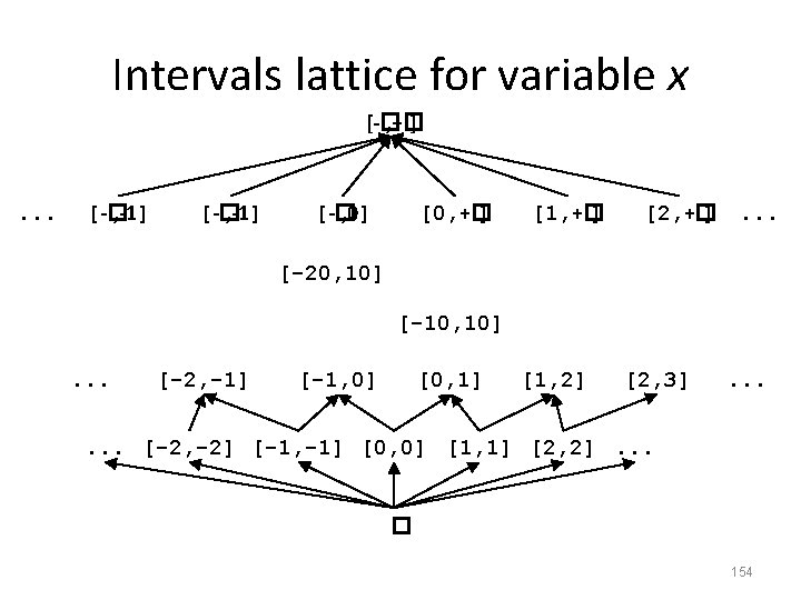
Intervals domain • One of the simplest numerical domains • Maintain for each variable x an interval [L, H] – L is either an integer of -� – H is either an integer of +� • A (non-relational) numeric domain 153

Intervals lattice for variable x • • Dint[x] = { (L, H) | L� -� , Z and H� Z, +�and L H} � � =[-� , +� ] �= ? – [1, 2] �[3, 4] ? – [1, 4] �[1, 3] ? – [1, 3] �[1, 4] ? – [1, 3] �[-� , +� ]? • What is the lattice height? 155

Intervals lattice for variable x • • Dint[x] = { (L, H) | L� -� , Z and H� Z, +�and L H} � � =[-� , +� ] �= ? – [1, 2] �[3, 4] no – [1, 4] �[1, 3] no – [1, 3] �[1, 4] yes – [1, 3] �[-� , +� ] yes • What is the lattice height? Infinite 156

Joining/meeting intervals • [a, b] �[c, d] = ? – [1, 1] �[2, 2] = ? – [1, 1] �[2, +� ]=? • [a, b] �[c, d] = ? – [1, 2] �[3, 4] = ? – [1, 4] �[3, 4] = ? – [1, 1] �[1, +� ]=? • Check that indeed x� y if and only if x� y=y 157

Joining/meeting intervals • [a, b] �[c, d] = [min(a, c), max(b, d)] – [1, 1] �[2, 2] = [1, 2] – [1, 1] �[2, +� ] = [1, +� ] • [a, b] �[c, d] = [max(a, c), min(b, d)] if a proper interval and otherwise � – [1, 2] �[3, 4] = � – [1, 4] �[3, 4] = [3, 4] – [1, 1] �[1, +� ] = [1, 1] • Check that indeed x� y if and only if x� y=y 158

Interval domain for programs • Dint[x] = { (L, H) | L� -� , Z and H� Z, +�and L H} • For a program with variables Var={x 1, …, xk} • Dint[Var] = ? 159

Interval domain for programs • • Dint[x] = { (L, H) | L� -� , Z and H� Z, +�and L H} For a program with variables Var={x 1, …, xk} Dint[Var] = Dint[x 1] �… �Dint[xk] How can we represent it in terms of formulas? 160

Interval domain for programs • • Dint[x] = { (L, H) | L� -� , Z and H� Z, +�and L H} For a program with variables Var={x 1, …, xk} Dint[Var] = Dint[x 1] �… �Dint[xk] How can we represent it in terms of formulas? – Two types of factoids x c and x c – Example: S = � {x 9, y 5, y 10} – Helper operations • c + +�= +� • remove(S, x) = S without any x-constraints • lb(S, x) = 161

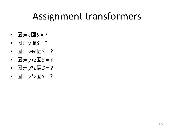
Assignment transformers � x : = c� # S = remove(S, x) �{x c, x c} � x : = y� # S = remove(S, x) �{x lb(S, y), x ub(S, y)} � x : = y+c� # S = remove(S, x) �{x lb(S, y)+c, x ub(S, y)+c} � x : = y+z� # S = remove(S, x) �{x lb(S, y)+lb(S, z), x ub(S, y)+ub(S, z)} • � x : = y*c� # S = remove(S, x) �if c>0 {x lb(S, y)*c, x ub(S, y)*c} else {x ub(S, y)*-c, x lb(S, y)*-c} • � x : = y*z� # S = remove(S, x) �? • • 163

assume transformers • • � assume x=c� #S=? � assume x<c� #S=? � assume x=y� #S=? � assume x c� #S=? 164

assume transformers • • � assume x=c� # S = S �{x c, x c} � assume x<c� # S = S �{x c-1} � assume x=y� # S = S �{x lb(S, y), x ub(S, y)} � assume x c� #S=? 165

assume transformers • • � assume x=c� # S = S �{x c, x c} � assume x<c� # S = S �{x c-1} � assume x=y� # S = S �{x lb(S, y), x ub(S, y)} � assume x c� # S = (S �{x c-1}) �(S �{x c+1}) 166

� Effect of function f on lattice elements • • • L = (D, � , � , � ) f : D D monotone Fix(f) = { d | f(d) = d } Red(f) = { d | f(d) d } Ext(f) = { d | d f(d) } Theorem [Tarski 1955] Red(f) fn (� ) gfp Fix(f) lfp Ext(f) – lfp(f) = Fix(f) = Red(f) Fix(f) – gfp(f) = Fix(f) = Ext(f) Fix(f) fn (� ) � 167

� Effect of function f on lattice elements • • • L = (D, � , � , � ) f : D D monotone Fix(f) = { d | f(d) = d } Red(f) = { d | f(d) d } Ext(f) = { d | d f(d) } Theorem [Tarski 1955] Red(f) fn (� ) gfp Fix(f) lfp Ext(f) – lfp(f) = Fix(f) = Red(f) Fix(f) – gfp(f) = Fix(f) = Ext(f) Fix(f) fn (� ) � 168

Continuity and ACC condition • Let L = (D, � , � ) be a complete partial order – Every ascending chain has an upper bound • A function f is continuous if for every increasing chain Y �D*, f(� Y) = � { f(y) | y� Y} • L satisfies the ascending chain condition (ACC) if every ascending chain eventually stabilizes: d 0 �d 1 �… �dn = dn+1 = … 169

Fixed-point theorem [Kleene] • Let L = (D, � , � ) be a complete partial order and a continuous function f: D D then n(� lfp(f) = � f ) n� N 170

Resulting algorithm • Kleene’s fixed point theorem gives a constructive method for computing the lfp � Mathematical definition n(� lfp(f) = � f ) n� N Algorithm d : = � while f(d) �d do d : = d �f(d) return d lfp fn(� ) … f 2(� ) f(� ) � 171

Chaotic iteration • Input: – – A cpo L = (D, � , � ) satisfying ACC Ln = L L … L A monotone function f : Dn Dn A system of equations { X[i] | f(X) | 1 i n } • Output: lfp(f) • A worklist-based algorithm for i: =1 to n do X[i] : = � WL = {1, …, n} while WL �do j : = pop WL // choose index non-deterministically N : = F[i](X) if N X[i] then X[i] : = N add all the indexes that directly depend on i to WL (X[j] depends on X[i] if F[j] contains X[i]) return X 172

Concrete semantics equations R[0] R[2] R[3] R[1] R[4] R[5] R[6] • R[0] = {x Z} R[1] = x: =7 R[2] = R[1] �R[4] R[3] = R[2] �{s | s(x) < 1000} R[4] = � x: =x+1 R[3] R[5] = R[2] {s | s(x) 1000} R[6] = R[5] �{s | s(x) 1001} 173

Abstract semantics equations R[0] R[2] R[3] R[1] R[4] R[5] R[6] • R[0] = ({x Z}) R[1] = x: =7 # R[2] = R[1] �R[4] R[3] = R[2] � ({s | s(x) < 1000}) R[4] = � x: =x+1 # R[3] R[5] = R[2] ({s | s(x) 1000}) R[6] = R[5] � ({s | s(x) 1001}) �R[5] � ({s | s(x) 999}) 174

Abstract semantics equations R[0] R[2] R[3] R[1] R[4] R[5] R[6] • R[0] = � R[1] = [7, 7] R[2] = R[1] �R[4] R[3] = R[2] �[-� , 999] R[4] = R[3] + [1, 1] R[5] = R[2] �[1000, +� ] R[6] = R[5] �[999, +� ] �R[5] �[1001, +� ] 175

Too many iterations to converge 176

How many iterations for this one? 177

Widening • Introduce a new binary operator to ensure termination – A kind of extrapolation • Enables static analysis to use infinite height lattices – Dynamically adapts to given program • Tricky to design • Precision less predictable then with finiteheight domains (widening non-monotone) 178

Formal definition • For all elements d 1 d 2 • For all ascending chains d 0 d 1 d 2 … the following sequence is finite – y 0 = d 0 – yi+1 = yi di+1 • For a monotone function f : D D define – x 0 = – xi+1 = xi f(xi ) • Theorem: – There exits k such that xk+1 = xk – xk Red(f) = { d | d D and f(d) d } 179

Analysis with finite-height lattice A Red(f) Fix(f) … f#n � = lpf(f#) � f#3� f#2 � f# � � 180

Analysis with widening A Red(f) f#2��f#3� lpf(f#) � Fix(f) f#3� f#2 � f# � � 181

Widening for Intervals Analysis • [c, d] = [c, d] • [a, b] [c, d] = [ if a c then a else - , if b d then b else 182

Semantic equations with widening R[0] R[2] R[3] R[1] R[4] R[5] R[6] • R[0] = � R[1] = [7, 7] R[2] = R[1] �R[4] R[2. 1] = R[2. 1] �R[2] R[3] = R[2. 1] �[-� , 999] R[4] = R[3] + [1, 1] R[5] = R[2] �[1001, +� ] R[6] = R[5] �[999, +� ] �R[5] �[1001, +� ] 183

Choosing analysis with widening Enable widening 184

Non monotonicity of widening • [0, 1] [0, 2] = ? • [0, 2] = ?

Non monotonicity of widening • [0, 1] [0, 2] = [0, ] • [0, 2] = [0, 2]

Analysis results with widening Did we prove it? 187

Analysis with narrowing A f#2��f#3� Red(f) lpf(f#) � Fix(f) f#3� f#2 � f# � � 188

Formal definition of narrowing • Improves the result of widening • y x y (x y) x • For all decreasing chains x 0 x 1 … the following sequence is finite – y 0 = x 0 – yi+1 = yi xi+1 • For a monotone function f: D D and xk Red(f) = { d | d D and f(d) d } define – y 0 = x – yi+1 = yi f(yi ) • Theorem: – There exits k such that yk+1 =yk – yk Red(f) = { d | d D and f(d) d }

Narrowing for Interval Analysis • [a, b] = [a, b] • [a, b] [c, d] = [ if a = - then c else a, if b = then d else b ]

Semantic equations with narrowing R[0] R[2] R[3] R[1] R[4] R[5] R[6] • R[0] = � R[1] = [7, 7] R[2] = R[1] �R[4] R[2. 1] = R[2. 1] �R[2] R[3] = R[2. 1] �[-� , 999] R[4] = R[3]+[1, 1] R[5] = R[2]# �[1000, +� ] R[6] = R[5] �[999, +� ] �R[5] �[1001, +� ] 191

Analysis with widening/narrowing • Two phases – Phase 1: analyze with widening until converging – Phase 2: use values to analyze with narrowing Phase 1: R[0] = � R[1] = [7, 7] R[2] = R[1] �R[4] R[2. 1] = R[2. 1] �R[2] R[3] = R[2. 1] �[-� , 999] R[4] = R[3] + [1, 1] R[5] = R[2] �[1001, +� ] R[6] = R[5] �[999, +� ] �R[5] �[1001, +� ] Phase 2: R[0] = � R[1] = [7, 7] R[2] = R[1] �R[4] R[2. 1] = R[2. 1] �R[2] R[3] = R[2. 1] �[-� , 999] R[4] = R[3]+[1, 1] R[5] = R[2]# �[1000, +� ] R[6] = R[5] �[999, +� ] �R[5] �[1001, +� ]192

Analysis with widening/narrowing 193

Analysis results widening/narrowing Precise invariant 194