Interprocedural Analysis Noam Rinetzky Mooly Sagiv Why do

Interprocedural Analysis Noam Rinetzky Mooly Sagiv

Why do runtime errors occur? • • • Logical errors Incorrect initializations Resource limitations Aliasing problems API mismatch 2

Procedural program void main() { int p(int a) { int x; x = p(7); x = p(9); } return a + 1; }

Effect of procedures foo() bar() call bar() The effect of calling a procedure is the effect of executing its body

Interprocedural Analysis foo() bar() call bar() goal: compute the abstract effect of calling a procedure

Reduction to intraprocedural analysis • Procedure inlining • Naive solution: call-as-goto

Reminder: Constant Propagation Variable not a constant - … -1 0 Z 1 … No information

Reminder: Constant Propagation • L = (Var Z , ) • 1 2 iff x: 1(x) ’ 2(x) – ’ ordering in the Z lattice • Examples: – [x , y 42, z ] [x , y 42, z 73] – [x , y 42, z 73] [x , y 42, z ]

Reminder: Constant Propagation • Conservative Solution – Every detected constant is indeed constant • But may fail to identify some constants – Every potential impact is identified • Superfluous impacts

Procedure Inlining void main() { int p(int a) { int x; x = p(7); x = p(9); } return a + 1; }

Procedure Inlining void main() { int p(int a) { int x; return a + 1; x = p(7); } x = p(9); } void main() { int a, x, ret; [a ⊥, x ⊥, ret ⊥] a = 7; ret = a+1; x = ret; [a 7, x 8, ret 8] a = 9; ret = a+1; x = ret; [a 9, x 10, ret 10] }

Procedure Inlining • Pros – Simple • Cons – Does not handle recursion – Exponential blow up – Reanalyzing the body of procedures p 1 { } p 2 { call p 2 call p 3 … … call p 2 call p 3 } p 3{ }

A Naive Interprocedural solution • Treat procedure calls as gotos

Simple Example void main() { int x ; x = p(7); x = p(9) ; } int p(int a) { return a + 1; }

Simple Example void main() { int p(int a) { [a 7] int x ; return a + 1; x = p(7); x = p(9) ; } }

Simple Example void main() { int p(int a) { [a 7] int x ; return a + 1; x = p(7); [a 7, $$ 8] x = p(9) ; } }

Simple Example void main() { int p(int a) { [a 7] int x ; return a + 1; x = p(7); [a 7, $$ 8] [x 8] x = p(9) ; [x 8] } }

Simple Example void main() { int p(int a) { [a 7] int x ; return a + 1; x = p(7); [a 7, $$ 8] [x 8] x = p(9) ; [x 8] } }

Simple Example void main() { int p(int a) { [a 7] [a 9] int x ; return a + 1; x = p(7); [a 7, $$ 8] [x 8] x = p(9) ; [x 8] } }

Simple Example void main() { int p(int a) { [a ] int x ; return a + 1; x = p(7); [a 7, $$ 8] [x 8] x = p(9) ; [x 8] } }

Simple Example void main() { int p(int a) { [a ] int x ; return a + 1; x = p(7); [a , $$ ] [x 8] x = p(9); [x 8] } }

Simple Example void main() { int p(int a) { [a ] int x ; return a + 1; x = p(7) ; [a , $$ ] [x ] x = p(9) ; [x ] } }

A Naive Interprocedural solution • Treat procedure calls as gotos • Pros: – Simple – Usually fast • Cons: – Abstract call/return correlations – Obtain a conservative solution

Analysis by reduction Procedure inlining Call-as-goto void main() { int p(int a) { void main() { int x ; [a ] int a, x, ret; x = p(7) ; return a + 1; [a ⊥, x ⊥, ret ⊥] [x ] [a , $$ ] a = 7; ret = a+1; x = ret; x = p(9) ; [a 7, x 8, ret 8] } [x ] a = 9; ret = a+1; x = ret; } [a 9, x 10, ret 10] } why was the naive solution less precise?

Stack regime ca P() { ca ll ll R(); rn } re rn tu re } … … R(); … R(){ tu … R P Q() { … }

Guiding light • Exploit stack regime Precision Efficiency

Simplifying Assumptions - Parameter passed by value - No procedure nesting - No concurrency ü Recursion is supported

Topics Covered ✓Procedure Inlining ✓The naive approach • Valid paths • The callstring approach • The Functional Approach • IFDS: Interprocedural Analysis via Graph Reachability • IDE: Beyond graph reachability • The trivial modular approach

Join-Over-All-Paths (JOP) • Let paths(v) denote the potentially infinite set paths from start to v (written as sequences of edges) • For a sequence of edges [e 1, e 2, …, en] define f [e 1, e 2, …, en]: L L by composing the effects of basic blocks f [e 1, e 2, …, en](l) = f(en) (… (f(e 2) (f(e 1) (l)) …) • JOP[v] = {f [e 1, e 2, …, en](l) | [e 1, e 2, …, en] paths(v)}

Join-Over-All-Paths (JOP) e 1 e 9 e 2 e 3 e 4 9 e 5 e 6 e 7 e 8 Paths transformers: f[e 1, e 2, e 3, e 4] f[e 1, e 2, e 7, e 8] f[e 5, e 6, e 3, e 4] f[e 1, e 2, e 3, e 4, e 9, e 1, e 2, e 3, e 4] f[e 1, e 2, e 7, e 8, e 9, e 1, e 2, e 3, e 4, e 9, …] … JOP: f[e 1, e 2, e 3, e 4](initial) f[e 1, e 2, e 7, e 8](initial) f[e 5, e 6, e 3, e 4](initial) … Number of program paths is unbounded due to loops

LFP approximates JOP • JOP[v] = {f [e 1, e 2, …, en](l) | [e 1, e 2, …, en] paths(v)} • LFP[v] = {f [e](LFP[v’]) | e =(v’, v)} LFP[v 0] = • JOP LFP - for a monotone function – f(x y) f(x) f(y) • JOP = LFP - for a distributive function – f(x y) = f(x) f(y) JOP may not be precise enough for interprocedural analysis!

Interprocedural analysis P R s. P Call node f 1 n 1 f 1 n 5 f 5 e. P Supergraph fx 2 r fc 2 e f 1 Call Q Return node s. R fc 2 e n 4 Entry node n 7 n 3 e. R f 1 Call node Call Q f 3 s. Q n 6 n 2 f 2 Q fx 2 r Exit node f 6 e. Q Return node

Paths s f 1 • paths(n) the set of paths from s to n – ( (s, n 1), (n 1, n 3), (n 3, n 1) ) n 1 f 1 n 2 f 3 n 3 f 3 e

Interprocedural Valid Paths f 2 callq f 1 f 3 ( enterq f 4 ret fk-1 ) fk fk-2 exitq fk-3 f 5 • IVP: all paths with matching calls and returns – And prefixes

Interprocedural Valid Paths • IVP set of paths – Start at program entry • Only considers matching calls and returns – aka, valid • Can be defined via context free grammar – matched : : = matched (i matched )i | ε – valid : : = valid (i matched | matched • paths can be defined by a regular expression

Join Over All Paths (JOP) i n start �fk o. . . o f 1� L L • JOP[v] = {[[e 1, e 2, …, en]](ι ) | (e 1, …, en) paths(v)} • JOP LFP – Sometimes JOP = LFP • precise up to “symbolic execution” • Distributive problem

The Join-Over-Valid-Paths (JVP) • vpaths(n) all valid paths from program start to n • JVP[n] = {[[e 1, e 2, …, e]](l) (e 1, e 2, …, e) vpaths(n)} • JVP JFP – In some cases the JVP can be computed – (Distributive problem)

The Call-String Approach • The data flow value is associated with sequences of calls (call string) • Use Chaotic iterations over the supergraph

Supergraph P R s. P Call node f 1 n 1 f 1 n 5 f 5 e. P fx 2 r fc 2 e f 1 Call Q Return node s. R fc 2 e n 4 Entry node n 7 n 3 e. R f 1 Call node Call Q f 3 s. Q n 6 n 2 f 2 Q fx 2 r Exit node f 6 e. Q Return node

Simple Example void main() { int p(int a) { int x ; return a + 1; c 1: x = p(7); c 2: x = p(9) ; } }

Simple Example void main() { int p(int a) { c 1: [a 7] int x ; return a + 1; c 1: x = p(7); c 2: x = p(9) ; } }

Simple Example void main() { int p(int a) { c 1: [a 7] int x ; return a + 1; c 1: x = p(7); c 1: [a 7, $$ 8] c 2: x = p(9) ; } }

Simple Example void main() { int p(int a) { c 1: [a 7] int x ; return a + 1; c 1: x = p(7); c 1: [a 7, $$ 8] : x 8 c 2: x = p(9) ; } }

Simple Example void main() { int p(int a) { c 1: [a 7] int x ; return a + 1; c 1: x = p(7); c 1: [a 7, $$ 8] : [x 8] c 2: x = p(9) ; } }

Simple Example void main() { int p(int a) { c 1: [a 7] c 2: [a 9] int x ; c 1: x = p(7); return a + 1; : [x 8] c 2: x = p(9) ; } c 1: [a 7, $$ 8] }

Simple Example void main() { int p(int a) { c 1: [a 7] c 2: [a 9] int x ; c 1: x = p(7); return a + 1; : [x 8] c 1: [a 7, $$ 8] c 2: [a 9, $$ 10] c 2: x = p(9) ; } }

Simple Example void main() { int p(int a) { c 1: [a 7] c 2: [a 9] int x ; c 1: x = p(7); return a + 1; : [x 8] c 1: [a 7, $$ 8] c 2: [a 9, $$ 10] c 2: x = p(9) ; : [x 10] } }

The Call-String Approach • The data flow value is associated with sequences of calls (call string) • Use Chaotic iterations over the supergraph • To guarantee termination limit the size of call string (typically 1 or 2) – Represents tails of calls • Abstract inline

Another Example (|cs|=2) void main() { int p(int a) { c 1: [a 7] c 2: [a 9] int x ; c 1: x = p(7); c 2. c 3: [b 10] return 2 * b; c 1: [a 7, $$ 16] c 2: [a 9, $$ 20] c 2: x = p(9) ; } c 1. c 3: [b 8] return c 3: p 1(a + 1); : [x 16] : [x 20] int p 1(int b) { c 1. c 3: [b 8, $$ 16] c 2. c 3: [b 10, $$ 20] } }

Another Example (|cs|=1) void main() { int p(int a) { c 1: [a 7] c 2: [a 9] int x ; c 1: x = p(7); return 2 * b; c 1: [a 7, $$ ] c 2: [a 9, $$ ] c 2: x = p(9) ; } (c 1|c 2)c 3: [b ] return c 3: p 1(a + 1); : [x ] int p 1(int b) { } (c 1|c 2)c 3: [b , $$ ] }

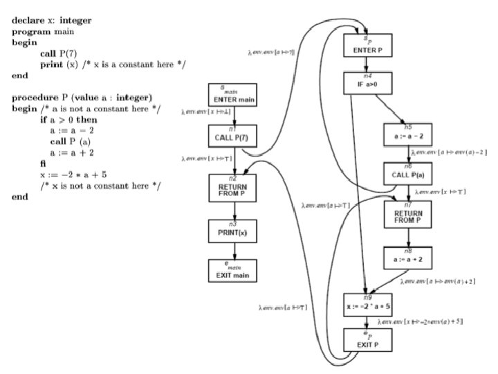
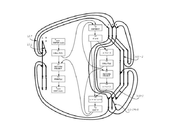
Handling Recursion void main() { int p(int a) { c 1: p(7); c 1: [a 7] : [x ] if (…) { } c 1. c 2+: [a ] c 1: [a 7] c 1. c 2+: [a ] a = a -1 ; c 1: [a 6] c 1. c 2+: [a ] c 2: p (a); c 1. c 2*: [a ] a = a + 1; c 1. c 2*: [a ] } c 1. c 2*: [a ] x = -2*a + 5; c 1. c 2*: [a , x ] }

Summary Call-String • Easy to implement • Efficient for very small call strings • Limited precision – Often loses precision for recursive programs – For finite domains can be precise even with recursion (with a bounded callstring) • Order of calls can be abstracted • Related method: procedure cloning

The Functional Approach • The meaning of a procedure is mapping from states into states • The abstract meaning of a procedure is function from an abstract state to abstract states • Relation between input and output • In certain cases can compute JVP

The Functional Approach • Two phase algorithm – Compute the dataflow solution at the exit of a procedure as a function of the initial values at the procedure entry (functional values) – Compute the dataflow values at every point using the functional values

Phase 1 void main() { p(7); } p(a 0, x 0) = [a a 0, x -2 a 0 + 5] int p(int a) { [a a 0, x x 0] if (…) { [a a 0, x x 0] a = a -1 ; [a a 0 -1, x x 0] p (a); [a a 0 -1, x 2 a 0+7] a = a + 1; [a a 0, x 2 a 0+7] } [a a 0, x x 0] ] x = -2*a + 5; [a a 0, x 2*a 0+5] }

Phase 2 void main() { p(7); [x -9] } int p(int a) { [a 7, x 0] if (…) { [a 7, x 0] a = a -1 ; [a 6, xx [a 0] 0] p (a); [a , x 0] [a 6, x -7] [a , x ] a = a + 1; [a 7, x -7] [a , x ] } [a 7, x [a , x ] 0] x = -2*a + 5; [a 7, x [a , x ] 9] p(a 0, x 0) = [a a 0, x -2 a 0 + 5] }

Tabulation for finite lattices L • Data facts: d L L • Initialization: – fstart, start= ( , ) ; otherwise ( , ) – S[start, ] = • Propagation of (x, y) over edge e = (n, n’) - - Maintain summary: S[n’, x] = S[n’, x] n, n’ (y)) - n intra-node: n’: (x, n, n’ (y)) - n call-node: n’: (y, y) if S[n’, y] = and n’= entry node n’: (x, z) if S[exit(call(n), y] = z and n’= ret-site-of n n return-node: n’: (u, y) ; nc = call-site-of n’, S[nc, u]=x

Issues in Functional Approach • How to guarantee that finite height for functional lattice? – It may happen that L has finite height and yet the lattice of monotonic function from L to L do not • Efficiently represent functions – Functional join – Functional composition – Testing equality

Summary Functional approach • • Computes procedure abstraction Sharing between different contexts Rather precise Recursive procedures may be more precise/efficient than loops • But requires more from the implementation – Representing (input/output) relations – Composing relations

CFL-Graph reachability [RHS’ 95] • Static analysis of programs with proecedures • Special cases of functional analysis • Reduce the interprocedural analysis problem to finding context free reachability [RHS’ 95] Thomas W. Reps, Susan Horwitz, Shmuel Sagiv: Precise Interprocedural Dataflow Analysis via Graph Reachability. POPL 1995

The Context-Free Reachability Problem • • • A finite directed graph G(s, V, E) A finite alphabet A labeling function l: E A context-free grammar C over A property holds at n N if there exists a path from s to n whose labels are in C 63

x y start main ( start p(a, b) if. x=3 p(x, y) a b . . Might by be uninitialized here? b=a p(a, b) return from p printf(y) printf(b) NO! YES! exit main ) exit p ]

Questions • When can we reduce a static analysis problem to CFL reachability • What is the complexity of solving CFL reachability problems • Interesting generalizations of CFL reachability

IFDS Problems • Finite subset distributive – – Lattice L = (D) is is Transfer functions are distributive • Efficient solution through formulation as CFL reachability • Can be generalized to certain infinite lattices

Possibly Uninitialized Variables {} Start {w, x, y} {w, y} x=3 if. . . {w, y} y=x {w, y} y=w {w} w=8 {} printf(y) {w, y}

Efficiently Representing Functions • Let f: 2 D 2 D be a distributive function • Then: – f(X) = { f({z}) | z X } – f(X) = f( ) { f({z}) | z X }

Encoding Transfer Functions • Enumerate all input space and output space • Represent functions as graphs with 2(D+1) nodes • Special symbol “ 0” denotes empty sets (sometimes denoted ) • Example: D = { a, b, c } f(S) = (S – {a}) U {b} 0 a b c

Representing Dataflow Functions Identity Function Constant Function a b c

Representing Dataflow Functions “Gen/Kill” Function Non-“Gen/Kill” Function a b c

Composing Dataflow Functions a b c

x y start main x=3 start p(a, b) if. a b . . b=a p(x, y) p(a, b) return from p printf(y) exit main printf(b) exit p

x y start main ( start p(a, b) if. x=3 p(x, y) a b . . Might by be uninitialized here? b=a p(a, b) return from p printf(y) printf(b) NO! YES! exit main ) exit p ]

The Tabulation Algorithm • Worklist algorithm, start from entry of “main” • Keep track of – Path edges: matched paren paths from procedure entry – Summary edges: matched paren call-return paths • At each instruction – Propagate facts using transfer functions; extend path edges • At each call – Propagate to procedure entry, start with an empty path – If a summary for that entry exits, use it • At each exit – Store paths from corresponding call points as summary paths – When a new summary is added, propagate to the return node

Asymptotic Running Time • CFL-reachability – Exploded control-flow graph: ND nodes – Running time: O(N 3 D 3) • Exploded control-flow graph Special structure Running time: O(ED 3) Typically: E N, hence O(ED 3) O(ND 3) “Gen/kill” problems: O(ED)

Some Applications Mayur Naik: Jchord a static analysis for Java IBM Watson: Wala static analysis tool Thomas Ball, Vladimir Levin, Sriram K. Rajaman A decade of software model checking with SLAM. CACM’ 11 Manu Sridharan, Rastislav Bodík: Refinement-based contextsensitive points-to analysis for Java. PLDI 2006 Nomair A. Naeem, Ondrej Lhoták, Jonathan Rodriguez: Practical Extensions to the IFDS Algorithm. CC 2010: 124 -144 Osbert Bastani, Saswat Anand, Alex Aiken: Specification Inference Using Context-Free Language Reachability, POPL’ 15 K Chatterjee, A Pavlogiannis, Y Velner: Quantitative interprocedural analysis, POPL’ 15 S Yang, D Yan, H Wu, Y Wang: Static control-flow analysis of userdriven callbacks in Android applications

Asymptotic Running Time • CFL-reachability – Exploded control-flow graph: ND nodes – Running time: O(N 3 D 3) • Exploded control-flow graph Special structure Running time: O(ED 3) Typically: E N, hence O(ED 3) O(ND 3) “Gen/kill” problems: O(ED)

IDE • Goes beyond IFDS problems – Can handle unbounded domains • Requires special form of the domain • Can be much more efficient than IFDS

Example Linear Constant Propagation • Consider the constant propagation lattice • The value of every variable y at the program exit can be represented by: y = {(axx + bx )| x Var* } c ax , c Z ∪{ , } bx Z • Supports efficient composition and “functional” join – [z : = a * y + b] – What about [z: =x+y]?

IDE Analysis • Point-wise representation closed under composition • CFL-Reachability on the exploded graph • Two phase algorithm – Compose functions – Compute dataflow values

Linear constant propagation Point-wise representation of environment transformers

Costs • O(ED 3) • Class of value transformers F L L – id F – Finite height • Representation scheme with (efficient) • • • Application Composition Join Equality Storage

Conclusion • Handling functions is crucial for abstract interpretation • Virtual functions and exceptions complicate things • But scalability is an issue – Small call strings – Small functional domains – Demand analysis

Bibliography • Textbook 2. 5 • Patrick Cousot & Radhia Cousot. Static determination of dynamic properties of recursive procedures In IFIP Conference on Formal Description of Programming Concepts, 1978 • Two Approaches to interprocedural analysis by Micha Sharir and Amir Pnueli: 1 • IDFS Interprocedural Distributive Finite Subset Precise interprocedural dataflow analysis via graph reachability. Reps, Horowitz, and Sagiv, POPL’ 95 • IDE Interprocedural Distributive Environment Precise interprocedural dataflow analysis with applications to constant propagation. Sagiv, Reps, Horowitz, and TCS’ 96