Program Analysis and Verification 0368 4479 Noam Rinetzky

Program Analysis and Verification 0368 -4479 Noam Rinetzky Lecture 6: Abstract Interpretation Slides credit: Roman Manevich, Mooly Sagiv, Eran Yahav

Abstract Interpretation [Cousot’ 77] • Mathematical foundation of static analysis 2

Abstract Interpretation [Cousot’ 77] • Mathematical foundation of static analysis – Abstract (semantic) domains (“abstract states”) – Transformer functions (“abstract steps”) – Chaotic iteration (“abstract computation”) 3

Abstract Interpretation [CC 77] • A very general mathematical framework for approximating semantics – Generalizes Hoare Logic – Generalizes weakest precondition calculus • Allows designing sound static analysis algorithms – Usually compute by iterating to a fixed-point – Not specific to any programming language style • Results of an abstract interpretation are (loop) invariants – Can be interpreted as axiomatic verification assertions and used for verification 4

Abstract Interpretation in 5 Slides • Disclaimer – Do not worry if you feel that you do not understand the next 5 slides • You are not expected to … – This is just to give you a view of the land …

Collecting semantics • For a set of program states State, we define the collecting lattice (2 State, � , � , State) • The collecting semantics accumulates the (possibly infinite) sets of states generated during the execution – Not computable in general 6

“Proof” x Z entry x Z if x>0 {x<=0} {x>0} x: = x + 1 {x>1} x : = x-1 {x<0} x : = x-1 {x<-1} 7

Abstract (conservative) interpretation abstract representation statement S abstract semantics concretization set of states abstract representation concretization statement S operational semantics (concrete semantics) set of states � set of states 8

Abstract (conservative) interpretation x = x -1 0<x abstract semantics concretization {x↦ 1, x↦ 2, …} 0≤x concretization x=x-1 operational semantics (concrete semantics) {x↦ 0, x↦ 1, …} �{x↦ 0, x↦ 1, …} 9

Abstract (conservative) interpretation x = x -1 0<x abstract semantics concretization {x↦ 1, x↦ 2, …} � concretization x=x-1 operational semantics (concrete semantics) {x↦ 0, x↦ 1, …} � {…, x↦ 0, …} 10

Abstract (non-conservative) interpretation x = x -1 0<x concretization {x↦ 1, x↦ 2, …} 0<x abstract semantics concretization x=x-1 operational semantics (concrete semantics) {x↦ 0, x↦ 1, …} ⊈ { x↦ 1, …} 11

Abstract Interpretation by Example

Available Expressions Analysis • A static analysis that infers for every program point a set of facts of the form AV = { x = y | x, y �Var } � { x = - y | x, y �Var } � { x = y op z | y, z �Var, op �{+, -, *, <=} } • For every program with n=|Var| variables number of possible facts is finite: |AV|=O(n 3) – Yields a trivial algorithm … but, is it efficient? 13

What do we need to prove? { true } C 1 x : = a op b C 2 { x = a op b } y : = a op b C 3 CSE { true } C 1 x : = a op b C 2 { x = a op b } y : = x C 3 14

Developing a theory of approximation • Formulae are suitable for many analysis-based proofs but we may want to represent predicates in other ways: – Sets of “facts” – Automata – Linear (in)equalities – … ad-hoc representation • Wanted: a uniform theory to represent semantic values and approximations 15

Preorder • We say that a binary order relation �over a set D is a preorder if the following conditions hold for every d, d’’ �D – Reflexive: d �d – Transitive: d �d’ and d’ �d’’ implies d �d’’ • There may exist d, d’ such that d �d’ and d’ �d yet d �d’ 16

Partial order • A binary order relation �over a set D is a partial order if – �is a preorder – �is anti-symmetric • For any d, d’ if d �d’ and d’ �d then d = d’ • Notation: if d �d’ and d �d’ we write d �d’ 17

Some posets-related terminology • If x �y we can say – x is lower than y – x is more precise than y – x is more concrete than y – x under-approximates y – y is greater than x – y is less precise than x – y is more abstract than x – y over-approximates x 18

Intuition • {x > 0} �x Z

Pointed poset • A poset (D, � ) with a least element �is called a pointed poset, and denoted by (D , � ) • For all d� D we have that ��d • We can always transform a poset (D, � ) into a pointed poset by adding a special bottom element (D �{� }, ��{� � d | d� D}, � ) 20

Join operator • Assume a poset (D, � ) • Let X �D be a subset of D (finite/infinite) • The join of X is defined as –� X = the least upper bound (LUB) of all elements in X if it exists –� X = min�{ b | forall x� X we have that x� b} – The supremum of the elements in X – A kind of abstract union (disjunction) operator • Properties of a join operator – Commutative: x �y = y �x – Associative: (x �y) �z = x �(y �z) – Idempotent: x �x = x 21

Join operator • Assume a poset (D, � ) • Let X �D be a subset of D (finite/infinite) • The join of X is defined as –� X = the least upper bound (LUB) of all elements in X if it exists –� X = min�{ b | forall x� X we have that x� b} – The supremum of the elements in X – A kind of abstract union (disjunction) operator • Properties of a join operator – Commutative: x �y = y �x – Associative: (x �y) �z = x �(y �z) – Idempotent: x �x = x 22

Meet operator • Assume a poset (D, � ) • Let X �D be a subset of D (finite/infinite) • The meet of X is defined as –� X = the greatest lower bound (GLB) of all elements in X if it exists –� X = max�{ b | forall x� X we have that b� x} – The infimum of the elements in X – A kind of abstract intersection (conjunction) operator • Properties of a join operator – Commutative: x �y = y �x – Associative: (x �y) �z = x �(y �z) – Idempotent: x �x = x 23

Meet operator • Assume a poset (D, � ) • Let X �D be a subset of D (finite/infinite) • The meet of X is defined as –� X = the greatest lower bound (GLB) of all elements in X if it exists –� X = max�{ b | forall x� X we have that b� x} – The infimum of the elements in X – A kind of abstract intersection (conjunction) operator • Properties of a join operator – Commutative: x �y = y �x – Associative: (x �y) �z = x �(y �z) – Idempotent: x �x = x 24

Complete lattices A complete lattice (D, � , � , � ) is A set of elements D A partial order x �y A join operator � A meet operator � A bottom element �= �D • A top element �= �D = �� • • • 25

Transfer Functions • Mathematical foundations

Towards an automatic proof • Goal: automatically compute an annotated program proving as many facts of the form x = y + z as possible • Decision 1: develop a forward-going proof • Decision 2: draw predicates from a finite set D – “looking under the light of the lamp” – A compromise that simplifies problem by focusing attention – possibly miss some facts that hold • Challenge 1: handle straight-line code • Challenge 2: handle conditions • Challenge 3: handle loops 27

Domain for SAV • Define atomic facts (for SAV) as = { x = y | x, y �Var } �{ x = y + z | x, y, z �Var } – For n=|Var| number of atomic facts is O(n 3) • Define sav-predicates as = 2 • For D � , Conj(D) = � D – Conj({a=b, c=b+d, b=c}) = (a=b) �(c=b+d) �(b=c) • Note: – Conj(D 1 �D 2) = Conj(D 1) �Conj(D 1) – Conj({}) �true 28

Visualizing ordering for SAV Greater {true} {x=y}* {y=z+a}* {p=q}* {x=y �y=z+a}* {x=y �p=q}* {y=z+a �p=q}* {false} D={x=y, y=x, p=q, q=p, y=z+a, y=a+z, z=y+z, x=z+a} Lower 29

An algorithm for annotating SLP • Annotate(P, x: =a) = {P} x: =a F*[x: =a](P) • Annotate(P, S 1; S 2) = {P} S 1; {Q 1} S 2 {Q 2 – Annotate(P, S 1) = {P} S 1 {Q 1} – Annotate(Q 1, S 2) = {Q 1} S 2 {Q 2} 30

handling conditions: Goal [ifp] { b �P } S 1 { Q }, { � b �P } S 2 { Q } { P } if b then S 1 else S 2 { Q } • Annotate a program if b then S 1 else S 2 with predicates from • Assumption 1: P is given (otherwise use true) • Assumption 2: b is a simple binary expression e. g. , x=y, x<y (why? ) {P} if b then { b �P } S 1 { Q 1 } else {� b �P } S 2 { Q 2 } {Q} 31

handling conditions: Goal [ifp] { b �P } S 1 { Q }, { � b �P } S 2 { Q } { P } if b then S 1 else S 2 { Q } • Annotate a program if b then S 1 else S 2 with predicates from • Assumption 1: P is given (otherwise use true) • Assumption 2: b is a simple binary expression e. g. , x=y, x<y (why? ) {P} if b then { b �P } S 1 { Q 1 } else {� b �P } S 2 { Q 2 } {Q} 32

Annotating conditions [ifp] { b �P } S 1 { Q }, { � b �P } S 2 { Q } { P } if b then S 1 else S 2 { Q } 1. Start with P or {b �P} and annotate S 1 (yielding Q 1) 2. Start with P or {� b �P} and annotate S 2 (yielding Q 2) 3. How do we infer a Q such that Q 1� Q and Q 2� Q? Q 1=Conj(D 1), Q 2 Possibly =Conj(D 2) an SAV-fact Define: Q = Q 1 �Q 2 = Conj(D 1 �D 2) Possibly an SAV-fact {P} if b then { b �P } S 1 { Q 1 } else {� b �P } S 2 { Q 2 } {Q} 33

Joining predicates [ifp] { b �P } S 1 { Q }, { � b �P } S 2 { Q } { P } if b then S 1 else S 2 { Q } 1. Start with P or {b �P} and annotate S 1 (yielding Q 1) 2. Start with P or {� b �P} and annotate S 2 (yielding Q 2) 3. How do we infer a Q such that Q 1� Q and Q 2� Q? Q 1=Conj(D 1), Q 2=Conj(D 2) Define: Q = Q 1 �Q 2 = Conj(D 1 �D 2) The join operator for SAV {P} if b then { b �P } S 1 { Q 1 } else {� b �P } S 2 { Q 2 } {Q} 34

Joining predicates • Q 1=Conj(D 1), Q 2=Conj(D 2) • We want to soundly approximate Q 1 �Q 2 in • Define: Q = Q 1 �Q 2 = Conj(D 1 �D 2) • Notice that Q 1� Q and Q 2� Q meaning Q 1 �Q 2 � Q 35

Handling conditional expressions • Let D be a set of facts and b be an expression • Goal: Elements in that soundly approximate – D �bexpr – D �� bexpr • Technique: Add statement assume bexpr sos s if B bexpr s = tt � assume bexpr, s�� • Find a function F[assume bexpr] : Conj(D) �bexpr �Conj(F[assume bexpr]) 36

Handling conditional expressions • F[assume bexpr] : such that Conj(D) �bexpr �Conj(F[assume bexpr]) • � (bexpr) = if bexpr is an SAV-fact then {bexpr} else {} – Notice bexpr �� (bexpr) – Examples • � (y=z) = {y=z} • � (y<z) = {} • F[assume bexpr](D) = D �� (bexpr) 37

Example { } if (x = y) { x=y, y=x } a : = b + c { x=y, y=x, a=b+c, a=c+b } d : = b – c { x=y, y=x, a=b+c, a=c+b } else { } a : = b + c { a=b+c, a=c+b } d : = b + c { a=b+c, a=c+b, d=b+c, d=c+b, a=d, d=a } { a=b+c, a=c+b } 38

Example { } if (x = y) { x=y, y=x } a : = b + c { x=y, y=x, a=b+c, a=c+b } d : = b – c { x=y, y=x, a=b+c, a=c+b } else { } a : = b + c { a=b+c, a=c+b } d : = b + c { a=b+c, a=c+b, d=b+c, d=c+b, a=d, d=a } { a=b+c, a=c+b } 39

Handling assumes • Meet or join?

Another Example

Constant Propagation (CP) • Goal: infers facts of the form x=c 42

Motivation: Constant folding • Optimization: constant folding { x=c } y : = aexpr constant folding simplifies constant expressions y : = eval(aexpr[c/x]) – Example: x: =7; y: =x*9 transformed to: x: =7; y: =7*9 and then to: x: =7; y: =63 43

CP semantic domain ? 44

CP semantic domain • Define CP-factoids: = { x = c | x �Var, c �Z } – How many factoids are there? • Define predicates as = 2 – How many predicates are there? – Do all predicates make sense? (x=5) �(x=7) • Treat conjunctive formulas as sets of factoids {x=5, y=7} ~ (x=5) �(y=7) 45

CP abstract transformer • Goal: define a function FCP[x: =aexpr] : such that if FCP[x: =aexpr] P = P’ then sp(x: =aexpr, P) �P’ ? 46

CP abstract transformer • Goal: define a function FCP[x: =aexpr] : such that if FCP[x: =aexpr] P = P’ then sp(x: =aexpr, P) �P’ [kill] { x=c } x: =aexpr { } [gen-1] { } x: =c { x=c } [gen-2] [preserve] { y=c, z=c’ } x: =y op z { x=c op c’ } { y=c } x: =aexpr { y=c } 47

Gen-kill formulation of transformers • Suited for analysis propagating sets of factoids – Available expressions, – Constant propagation, etc. • For each statement, define a set of killed factoids and a set of generated factoids F[S] P = (P kill(S)) �gen(S) • FCP[x: =aexpr] P = (P {x=c}) aexpr is not a constant • FCP[x: =k] P = (P {x=c}) �{x=k} • Used in dataflow analysis – a special case of abstract interpretation 48

Does this still work? Annotate(P, S 1; S 2) = let Annotate(P, S 1) be {P} A 1 {Q 1} let Annotate(Q 1, S 2) be {Q 1} A 2 {Q 2} return {P} A 1; {Q 1} A 2 {Q 2} 49

Handling conditional expressions • We want to soundly approximate D �bexpr and D �� bexpr in • Define an artificial statement assume bexpr sos s if B bexpr s = tt � assume bexpr, s�� • Define � (bexpr) = if bexpr is CP-factoid {bexpr} else {} • Define F[assume bexpr](D) = D �� (bexpr) 50

Does this still work? let Pt = F[assume bexpr] P let Pf = F[assume � bexpr] P let Annotate(Pt, S 1) be {Pt} S 1 {Q 1} let Annotate(Pf, S 2) be {Pf} S 2 {Q 2} return {P} if bexpr then {Pt} S 1 {Q 1} else {Pf} S 2 {Q 2} {Q 1 �Q 2} How do we define join for CP? 51

Join example • {x=5, y=7} �{x=3, y=7, z=9} = 52

Does this still work? Annotate(P, while bexpr do S) = N’ : = Nc : = P // Initialize repeat let Pt = F[assume bexpr] Nc let Annotate(Pt, S) be {Nc} Abody {N’} Nc : = Nc �N’ until N’ = Nc return {P} INV= {N’} while bexpr do {Pt} Abody {F[assume � bexpr](N)} • What about correctness? • What about termination? 53

Does this still work? Annotate(P, while bexpr do S) = N’ : = Nc : = P // Initialize repeat let Pt = F[assume bexpr] Nc let Annotate(Pt, S) be {Nc} Abody {N’} Nc : = Nc �N’ until N’ = Nc return {P} INV= {N’} while bexpr do {Pt} Abody {F[assume � bexpr](N)} • What about correctness? – If loop terminates then is N’ a loop invariant? • What about termination? 54

What were the common elements? • Two static analyses – Available Expressions (extended with equalities) – Constant Propagation • Semantic domain – An approximation relation � • A weaker one given by set inclusion – Join operator • Abstract transformers for basic statements – Assignments – assume statements • Initial precondition 55

Abstract Interpretation [Cousot’ 77] More Formally … • Mathematical foundation of static analysis 56

Abstract Interpretation [Cousot’ 77] • Mathematical framework for approximating semantics (aka abstraction) – Allows designing sound static analysis algorithms • Usually compute by iterating to a fixed-point – Computes (loop) invariants • Can be interpreted as axiomatic verification assertions • Generalizes Hoare Logic & WP / SP calculus 57

Abstract Interpretation [Cousot’ 77] • Mathematical foundation of static analysis – Abstract domains • Abstract states ~ Assertions • Join (� ) ~ Weakening – Transformer functions • Abstract steps ~ Axioms – Chaotic iteration • Structured Programs ~ Control-flow graphs • Abstract computation ~ Loop invariants 58

Introduction to Domain Theory 60

Motivation • Let “isone” be a function that must return “ 1$” when the input string has at least a 1 and “ 0$” otherwise – isone(00… 0$) = 0$ – isone(xx… 1…$) =1$ – isone(0… 0) =? • Monotonicity: in terms of information – Output is never retracted • More information about the input is reflected in more information about the output – How do we express monotonicity precisely? 61

Montonicity • Define a partial order x �y – A partial order is reflexive, transitive, and anti-symmetric – y is a refinement of x • “more precise” • For streams of bits x � y when x is a prefix of y • For programs, a typical order is: – No output (yet) �some output 62

Montonicity • A set equipped with a partial order is a poset • Definition: – D and E are postes – A function f: D E is monotonic if x, y D: x � D y f(x) � E f(y) – The semantics of the program ought to be a monotonic function • More information about the input leads to more information about the output 63

Montonicity Example • Consider our “isone” function with the prefix ordering • Notation: – 0 k is the stream with k consecutive 0’s – 0 is the infinite stream with only 0’s • Question (revisited): what is isone(0 k )? – By definition, isone(0 k$) = 0$ and isone(0 k 1$) = 1$ – But 0 k� 0 k$ and 0 k � 0 k 1$ – “isone” must be monotone, so: • isone( 0 k ) �isone( 0 k$) = 0$ • isone( 0 k ) �isone( 0 k 1$) = 1$ – Therefore, monotonicity requires that isone(0 k ) is a common prefix of 0$ and 1$, namely 64

Motivation • Are there other constraints on “isone”? • Define “isone” to satisfy the equations – – isone( )= isone(1 s)=1$ isone(0 s)=isone(s) isone($)=0$ • What about 0 ? • Continuity: finite output depends only on finite input (no infinite lookahead) – Intuition: A program that can produce observable results can do it in a finite time 65

Chains • A chain is a countable increasing sequence <xi> = {xi X | x 0 � x 1 �… } • An upper bound of a set if an element “bigger” than all elements in the set • The least upper bound is the “smallest” among upper bounds: – xi �� <xi> for all i N – � <xi> � y for all upper bounds y of <xi> and it is unique if it exists 66

Complete Partial Orders • Not every poset has an upper bound – with ��n and n� n for all n N – {1, 2} does not have an upper bound 0 1 2 … � • Sometimes chains have no upper bound � 2 The chain 1 0 1 2 … 0 does not have an upper bound 67

Complete Partial Orders • It is convenient to work with posets where every chain (not necessarily every set) has a least upper bound • A partial order P is complete if every chain in P has a least upper bound also in P • We say that P is a complete partial order (cpo) • A cpo with a least (“bottom”) element �is a pointed cpo (pcpo) 68

Examples of cpo’s • Any set P with the order x� y if and only if x = y is a cpo It is discrete or flat • If we add �so that �� x for all x P, we get a flat pointed cpo • The set N with is a poset with a bottom, but not a complete one • The set N { } with n is a pointed cpo • The set N with is a cpo without bottom • Let S be a set and P(S) denotes the set of all subsets of S ordered by set inclusion – P(S) is a pointed cpo 69

Constructing cpos • If D and E are pointed cpos, then so is D×E (x, y) �D×E (x’, y’) iff x � D x’ and y� E y’ � D×E = (� D, � E) �(x i , y i ) = ( � D xi , � E y i) 70

Constructing cpos (2) • If S is a set of E is a pcpos, then so is S E m �m’ iff s S: m(s) � E m’(s) � S E = s. � E �(m , m’ ) = s. m(s) � E m’(s) 71

Continuity • A monotonic function maps a chain of inputs into a chain of outputs: x 0 �x 1 � … f(x 0) �f(x 1) �… • It is always true that: � f(� i <f(xi)> � i <xi>) • But f(� � i <xi>)� i <f(xi)> is not always true 72

A Discontinuity Example � 3 2 1 f(� � i <xi>) � i <f(xi)> 1 0 73

Continuity • Each f(xi) uses a “finite” view of the input • f(� <xi> ) uses an “infinite” view of the input • A function is continuous when f(� <xi>) = � i <f(xi)> • The output generated using an infinite view of the input does not contain more information than all of the outputs based on finite inputs 74

Continuity • Each f(xi) uses a “finite” view of the input • f(� <xi> ) uses an “infinite” view of the input • A function is continuous when f(� <xi>) = � i <f(xi)> • The output generated using an infinite view of the input does not contain more information than all of the outputs based on finite inputs • Scott’s thesis: The semantics of programs can be described by a continuous functions 75

Examples of Continuous Functions • For the partial order ( N { }, ) – The identity function is continuous id(� ni) = � id(ni ) – The constant function “five(n)=5” is continuous five(� ni) = � five(ni ) – If isone(0 ) = then isone is continuos • For a flat cpo A, any monotonic function f: A� A� such that f is strict is continuous • Chapter 8 of the Wynskel textbook includes many more continuous functions 76

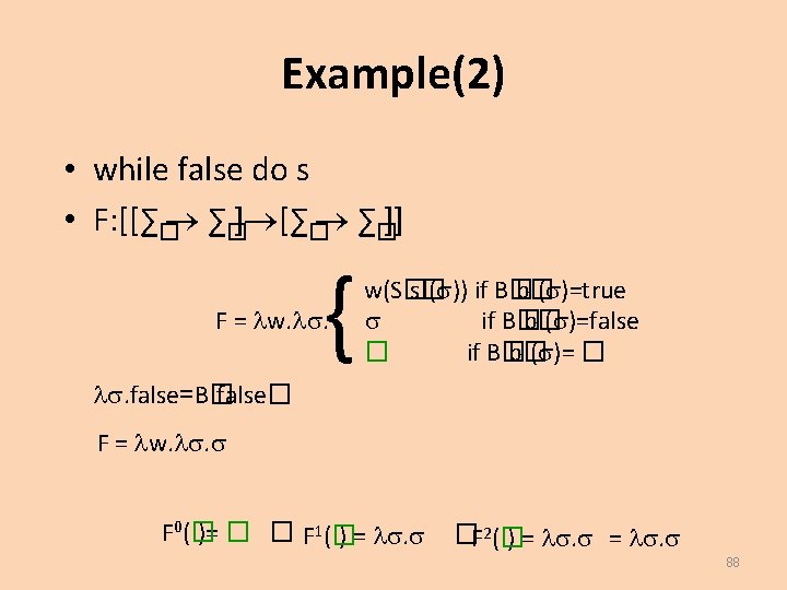
Fixed Points • Solve equation: { W(S� s� ) if B� b� ( )=true W( ) = if B� b� ( )=false � if B� b� ( )= � where W: ∑� ∑�; W= S� while b do S� 77

Fixed Points • Solve equation: { W(S� s� ) if B� b� ( )=true W( ) = if B� b� ( )=false � if B� b� ( )= � where W: ∑� ∑�; W= S� while be do s� • Alternatively, W = F(W) where: F(W) = . { W(S� s� ) if B� b� ( )=true if B� b� ( )=false � if B� b� ( )= � 78

Fixed Point (cont) • Thus we are looking for a solution for W = F( W) – a fixed point of F • Typically there are many fixed points • We may argue that W ought to be continuous W [∑� ∑�] • Cut the number of solutions • We will see how to find the least fixed point for such an equation provided that F itself is continuous 79

Fixed Point Theorem • • Define Fk = x. F( F(… F( x)…)) (F composed k times) If D is a pointed cpo and F : D D is continuous, then – – • for any fixed-point x of F and k N Fk (� ) �x The least of all fixed points is k ) � k F (� Proof: i. By induction on k. • • Base: F 0 (�) = ��x Induction step: Fk+1 (�) = F( Fk (�)) �F( x) = x k ) is a fixed-point ii. It suffices to show that � k F (� • k )) = �Fk+1 ( � k ) F(� )=� k F (� k k F (� 80

Fixed-Points (notes) • If F is continuous on a pointed cpo, we know how to find the least fixed point • All other fixed points can be regarded as refinements of the least one – They contain more information, they are more precise – In general, they are also more arbitrary 81

Fixed-Points (notes) • If F is continuous on a pointed cpo, we know how to find the least fixed point • All other fixed points can be regarded as refinements of the least one – They contain more information, they are more precise – In general, they are also more arbitrary – They also make less sense for our purposes 82

Denotational Semantics • Meaning of programs

Denotational Semantics of While • ∑�is a flat pointed cpo – A state has more information on non-termination – Otherwise, the states must be equal to be comparable (informationwise) • We want strict functions ∑� ∑� – therefore, continuous functions • The partial order on ∑� ∑� f �g iff f(x) =�or f(x) = g(x) for all x ∑� – g terminates with the same state whenever f terminates – g might terminate for more inputs 84

Denotational Semantics of While • Recall that W is a fixed point of F: [[∑� ∑�]] • F is continuous { F(w) = . w(S� s� ( )) if B� b� ( )=true if B� b� ( )=false � if B� b� ( )= � • Thus, we set S� while b do c�= � Fk(� ) – Least fixed point • Terminates least often of all fixed points • Agrees on terminating states with all fixed point 85

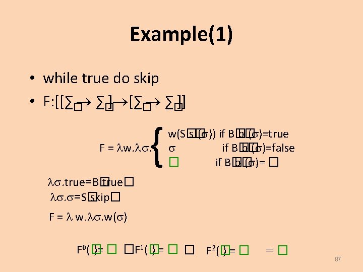
Denotational Semantics of While • S� skip�= . • S� X : = exp�= . [X �A� exp � ] • S� s 0 ; s 1 � = . S � s 1 � (S � s 0 � ) • S� if b then s 0 else s 1� = . if B� b� then S � s 0 � else S � s 1 � • S �while b do s�= � Fk(� ) – k=0, 1, … – F = w. . if B� b� ( )=true w(S� s� ( )) else 86

Example(3) �while x 3 do x = x -1 �= � Fk(� ) k=0, 1, … where F = w. . if (x) 3 w( [x � (x) -1]) else F 0(� ) � F 1(� ) if (x) 3 � ( [x � (x) -1]) else if (x) 3 then �else F 2(� ) if if Fk(� ) lfp(F) if (x) {3, 4, …k} then [x � 3] else � if (x) 3 then [x � 3] else � (x) 3 then F 1( [x � (x) -1] ) else (x) 3 then (if [x � (x) -1] x 3 then �else [x � (x) -1] ) else (x) 3 (if (x) 4 then �else [x � (x) -1] ) else (x) {3, 4} then [x � 3] else � 89

Complete Lattice • Let (D, � ) be a partial order • D is a complete lattice if every subset has both greatest lower bounds and least upper bounds 90

Knaster-Tarski Theorem • Let f: L L be a monotonic function on a complete lattice L • The least fixed point lfp(f) exists – lfp(f) = � {x L: f(x)� x} 91

Fixed Points � f(� ) f 2(� ) • A monotone function f: L L where (L, � , � , � ) is a complete lattice • Fix(f) = { l: l �L, f(l) = l} • Red(f) = {l: l �L, f(l) �l} • Ext(f) = {l: l �L, l �f(l)} Red(f) gfp(f) Fix(f) – l 1 �l 2 f(l 1 ) �f(l 2 ) • Tarski’s Theorem 1955: if f is monotone then: – lfp(f) = �Fix(f) = �Red(f) �Fix(f) – gfp(f) = �Fix(f) = �Ext(f) �Fix(f) Ext(f) lfp(f) f 2(� ) f(� ) � 92

Constant Propagation - Again

Constant Propagation • Optimization: constant folding { x=c } y : = aexpr simplifies constant expressions y : = eval(aexpr[c/x]) – Example: x: =7; y: =x*9 transformed to: x: =7; y: =7*9 and then to: x: =7; y: =63 • Analysis: constant propagation (CP) – Infers facts of the form x=c 94

CP semantic domain • Define CP-factoids: = { x = c | x �Var, c �Z } – How many factoids are there? • Define predicates as = 2 – How many predicates are there? – Do all predicates make sense? (x=5) �(x=7) • Treat conjunctive formulas as sets of factoids {x=5, y=7} ~ (x=5) �(y=7) 95

One lattice per variable true x� 0 x<0 true x� 0 x=0 false y� 0 x>0 y<0 y� 0 y=0 y>0 false How can we compose them? 96

Cartesian product of complete lattices • For two complete lattices L 1 = (D 1, � 1, � 1) L 2 = (D 2, � 2, � 2) • Define the poset Lcart = (D 1 D 2, � cart, � cart) as follows: – (x 1, x 2) � cart (y 1, y 2) iff x 1 � 1 y 1 x 2 � 2 y 2 –� � cart = ? • Lemma: L is a complete lattice • Define the Cartesian constructor Lcart = Cart(L 1, L 2) 97

Cartesian product example � =(� , � ) x� 0, y� 0 x� 0, y� 0 … x� 0, y� 0 x� 0, y<0 x� 0, y=0 x� 0, y>0 x<0, y<0 x<0, y=0 x<0, y>0 x=0, y<0 x=0, y=0 x=0, y>0 How does it represent (x<0� y<0) �(x>0� y>0)? … y� 0 x� 0, y� 0 … x>0, y<0 x>0, y� 0 x>0, y=0 x>0, y>0 � =(� , � ) (false, false) 98

Disjunctive completion • For a complete lattice L = (D, � , � , � ) • Define the powerset lattice L�= (2 D, � , � , � ) � � �= ? �= ? • Lemma: L�is a complete lattice • L�contains all subsets of D, which can be thought of as disjunctions of the corresponding predicates • Define the disjunctive completion constructor L�= Disj(L) 99

The base lattice CP � … {x=-2} {x=-1} {x=0} {x=1} {x=2} … � 100

The disjunctive completion of CP What is the height of this lattice? … … {x=-2} {x=-2� x=-1} {x=-1} true {x=0} {x=-2� x=0} … {x=1} {x=-2� x=1} {x=-1�x=1� x=-2} … … {x=2} … … … {x=1� x=2} {x=0�x=1� x=2} … false 101

Relational product of lattices • L 1 = (D 1, � 1, � 1) L 2 = (D 2, � 2, � 2) • Lrel = (2 D 1 D 2, � rel, � rel) as follows: – Lrel = ? 102

Relational product of lattices • L 1 = (D 1, � 1, � 1) L 2 = (D 2, � 2, � 2) • Lrel = (2 D 1 D 2, � rel, � rel) as follows: – Lrel = Disj(Cart(L 1, L 2)) • Lemma: L is a complete lattice • What does it buy us? 103

Cartesian product example true x� 0, y� 0 x� 0, y� 0 … x� 0, y� 0 x� 0, y<0 x� 0, y=0 x� 0, y>0 x<0, y<0 x<0, y=0 x<0, y>0 x=0, y<0 x=0, y=0 x=0, y>0 How does it represent (x<0� y<0) �(x>0� y>0)? … false y� 0 … x>0, y<0 x>0, y� 0 x>0, y=0 x>0, y>0 What is the height of this lattice? 104

Relational product example true x� 0 (x<0� y<0)� (x>0� y>0) y� 0 (x<0� y<0)� (x>0� y=0) y� 0 (x<0� y� 0)� (x<0� y� 0) … How does it represent (x<0� y<0) �(x>0� y>0)? false What is the height of this lattice? 105