PCFG estimation with EM The InsideOutside Algorithm Presentation

PCFG estimation with EM The Inside-Outside Algorithm

Presentation order l l l Notation Calculating inside probabilities Calculating outside probabilities General schema for EM algorithms The inside-outside algorithm

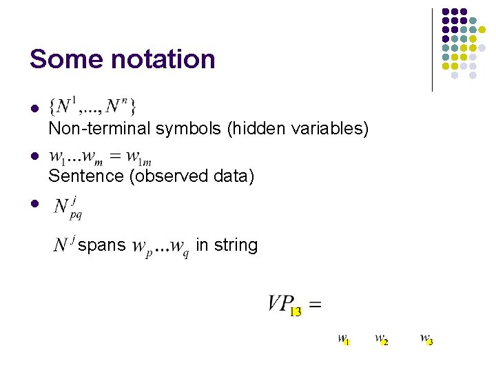
Some notation l Non-terminal symbols (hidden variables) l Sentence (observed data) l spans in string

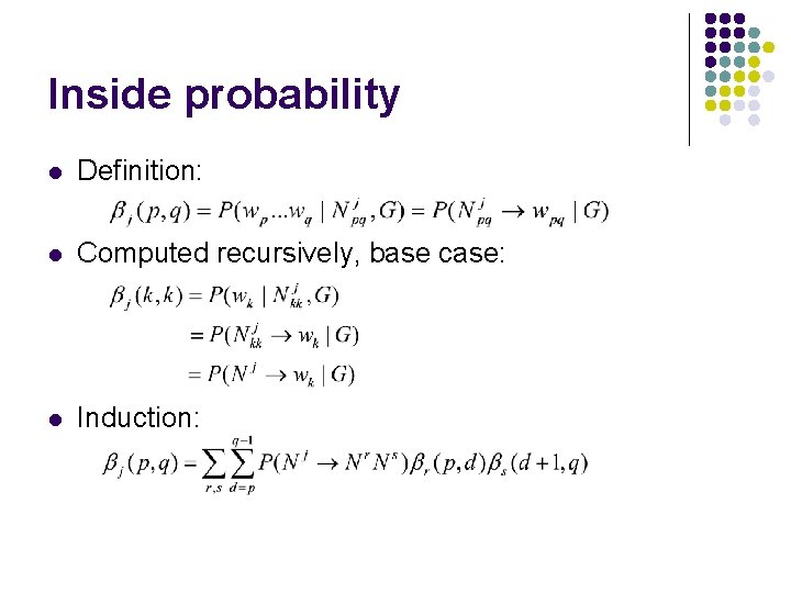
Inside probability l Definition: l Computed recursively, base case: l Induction:

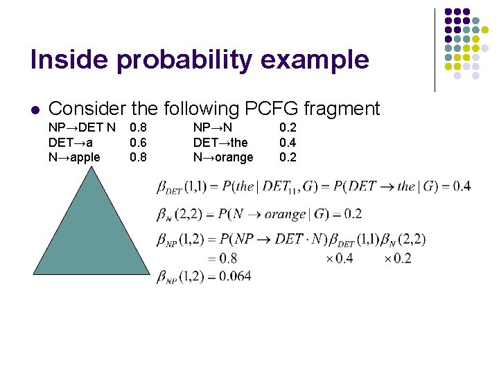
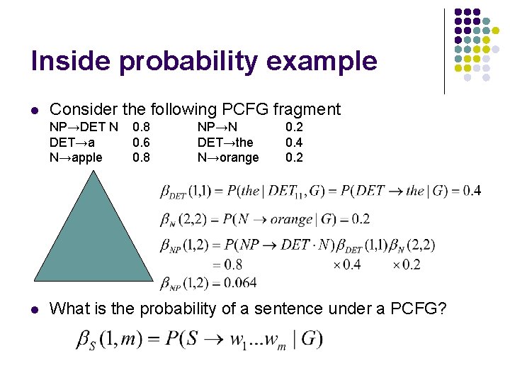
Inside probability example l Consider the following PCFG fragment NP→DET N DET→a N→apple 0. 8 0. 6 0. 8 NP→N DET→the N→orange 0. 2 0. 4 0. 2

Inside probability example l Consider the following PCFG fragment NP→DET N DET→a N→apple l 0. 8 0. 6 0. 8 NP→N DET→the N→orange 0. 2 0. 4 0. 2 What is the probability of a sentence under a PCFG?

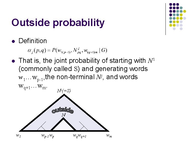
Outside probability l Definition l That is, the joint probability of starting with N 1 (commonly called S) and generating words w 1…wp-1, the non-terminal Nj, and words wq+1…wm. N 1(=S) Nj w 1 wp-1 wp wqwq+1 wm

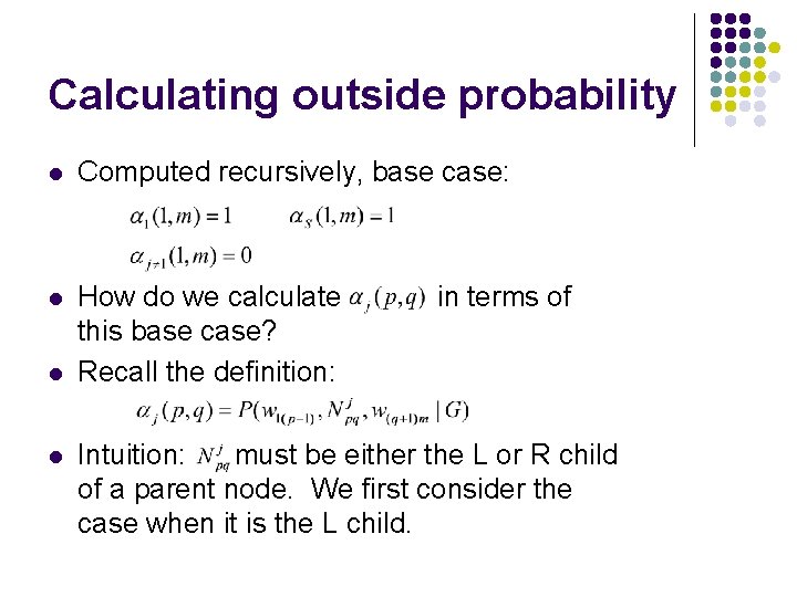
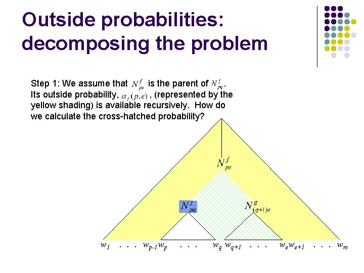
Calculating outside probability l Computed recursively, base case: l How do we calculate this base case? Recall the definition: l l in terms of Intuition: must be either the L or R child of a parent node. We first consider the case when it is the L child.

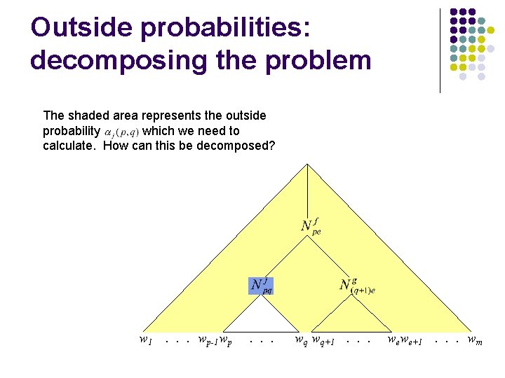
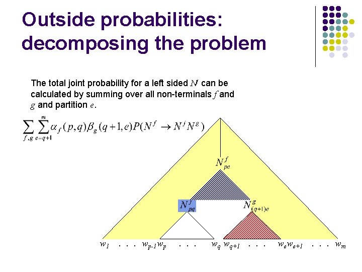
Outside probabilities: decomposing the problem The shaded area represents the outside probability which we need to calculate. How can this be decomposed? w 1 . . . wp-1 wp . . . wq wq+1. . . we we+1. . . wm

Outside probabilities: decomposing the problem Step 1: We assume that is the parent of. Its outside probability, , (represented by the yellow shading) is available recursively. How do we calculate the cross-hatched probability? w 1 . . . wp-1 wp . . . wq wq+1. . . we we+1. . . wm

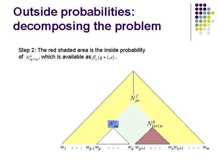
Outside probabilities: decomposing the problem Step 2: The red shaded area is the inside probability of , which is available as. w 1 . . . wp-1 wp . . . wq wq+1. . . we we+1. . . wm

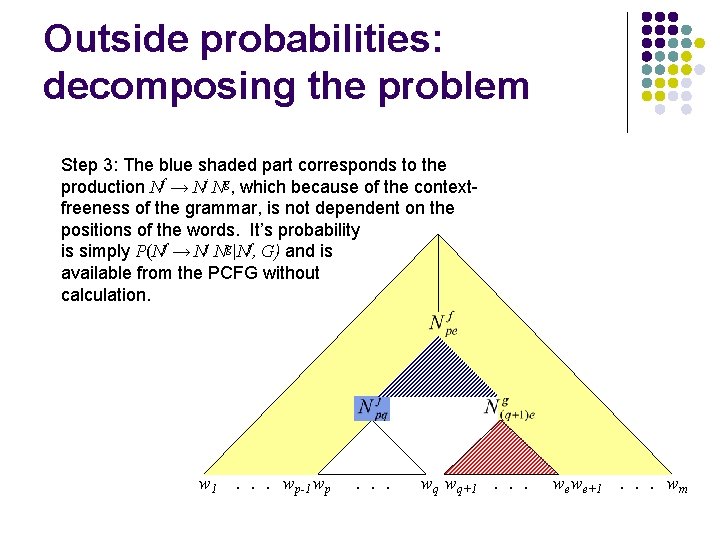
Outside probabilities: decomposing the problem Step 3: The blue shaded part corresponds to the production Nf → Nj Ng, which because of the contextfreeness of the grammar, is not dependent on the positions of the words. It’s probability is simply P(Nf → Nj Ng|Nf, G) and is available from the PCFG without calculation. w 1 . . . wp-1 wp . . . wq wq+1. . . we we+1. . . wm

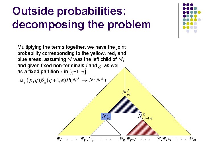
Outside probabilities: decomposing the problem Multiplying the terms together, we have the joint probability corresponding to the yellow, red, and blue areas, assuming Nj was the left child of Nf, and given fixed non-terminals f and g, as well as a fixed partition e in [q+1, m]. w 1 . . . wp-1 wp . . . wq wq+1. . . we we+1. . . wm

Outside probabilities: decomposing the problem The total joint probability for a left sided Nj can be calculated by summing over all non-terminals f and g and partition e. w 1 . . . wp-1 wp . . . wq wq+1. . . we we+1. . . wm

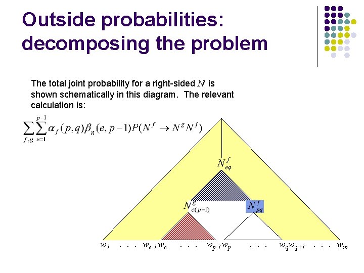
Outside probabilities: decomposing the problem The total joint probability for a right-sided Nj is shown schematically in this diagram. The relevant calculation is: w 1 . . . we-1 we . . . wp-1 wp . . . wqwq+1. . . wm

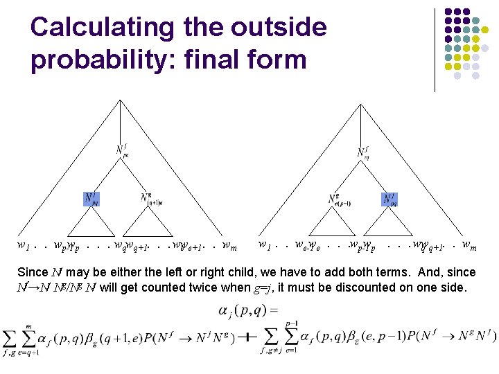
Calculating the outside probability: final form w 1. . . wp-1 wp. . . wqwq+1. . . ww e e+1. . . wm w 1. . . we-1 we. . . wp-1 wp. . . ww q q+1. . . wm Since Nj may be either the left or right child, we have to add both terms. And, since Nf→Nj Ng/Ng Nj will get counted twice when g=j, it must be discounted on one side.

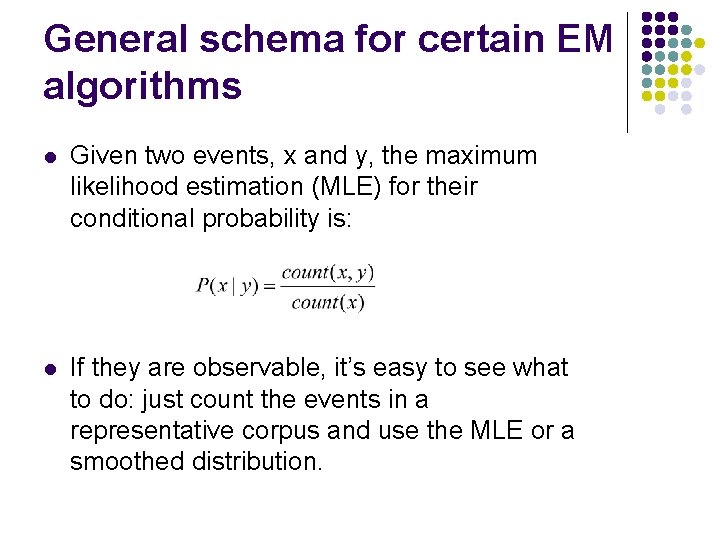
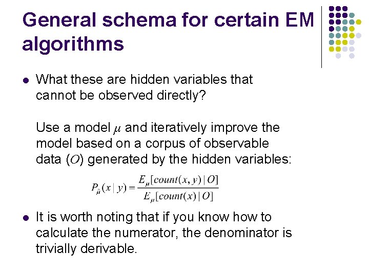
General schema for certain EM algorithms l Given two events, x and y, the maximum likelihood estimation (MLE) for their conditional probability is: l If they are observable, it’s easy to see what to do: just count the events in a representative corpus and use the MLE or a smoothed distribution.

General schema for certain EM algorithms l What these are hidden variables that cannot be observed directly? Use a model μ and iteratively improve the model based on a corpus of observable data (O) generated by the hidden variables: l It is worth noting that if you know how to calculate the numerator, the denominator is trivially derivable.

General schema for certain EM algorithms l By updating μ and iterating, the model converges to at least a local maximum. l This can be proven, but I will not do it here.

The inside-outside algorithm l Goal: estimate a model μ that is a PCFG (in Chomsky normal form) that characterizes a corpus of text. l Required input: l l Size of non-terminal vocabulary, n At least one sentence to be modeled, O

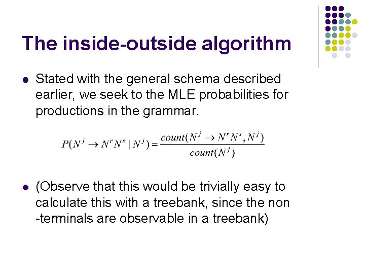
The inside-outside algorithm l Stated with the general schema described earlier, we seek to the MLE probabilities for productions in the grammar. l (Observe that this would be trivially easy to calculate this with a treebank, since the non -terminals are observable in a treebank)

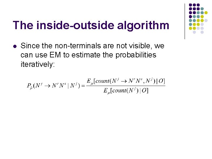
The inside-outside algorithm l Since the non-terminals are not visible, we can use EM to estimate the probabilities iteratively:

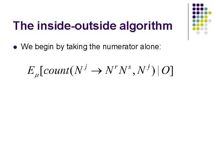
The inside-outside algorithm l We begin by taking the numerator alone:

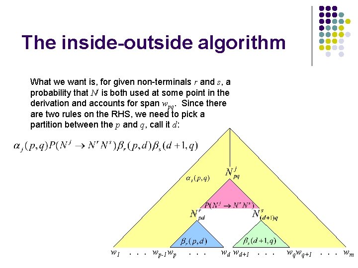
The inside-outside algorithm What we want is, for given non-terminals r and s, a probability that Nj is both used at some point in the derivation and accounts for span wpq. Since there are two rules on the RHS, we need to pick a partition between the p and q, call it d: w 1 . . . wp-1 wp . . . wd wd+1. . . wqwq+1. . . wm

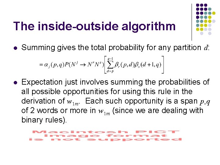
The inside-outside algorithm l Summing gives the total probability for any partition d: l Expectation just involves summing the probabilities of all possible opportunities for using this rule in the derivation of w 1 m. Each such opportunity is a span p, q of 2 words or more in w 1 m (since we are dealing with binary rules).

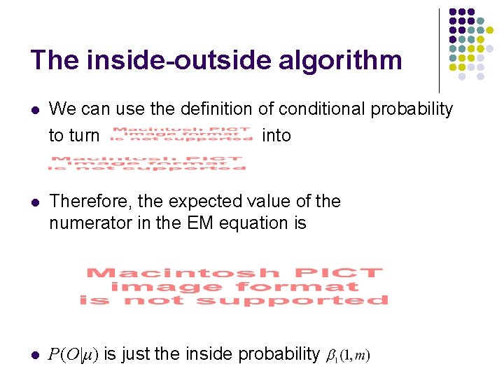
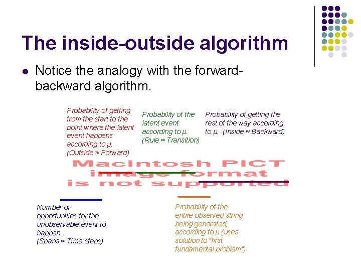
The inside-outside algorithm l We can use the definition of conditional probability to turn into l Therefore, the expected value of the numerator in the EM equation is l P(O|μ) is just the inside probability

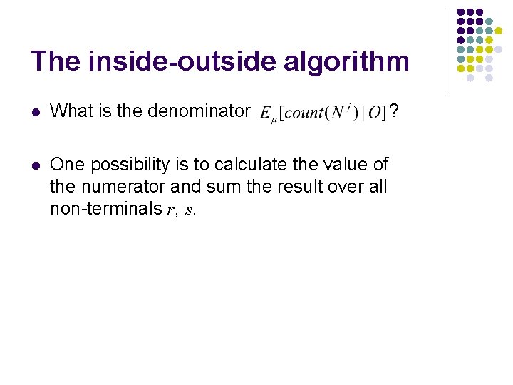
The inside-outside algorithm l Notice the analogy with the forwardbackward algorithm. Probability of getting from the start to the point where the latent event happens according to μ. (Outside ≈ Forward) Number of opportunities for the unobservable event to happen. (Spans ≈ Time steps) Probability of the Probability of getting the latent event rest of the way according to μ. (Inside ≈ Backward) (Rule ≈ Transition) Probability of the entire observed string being generated, according to μ (uses solution to “first fundamental problem”)

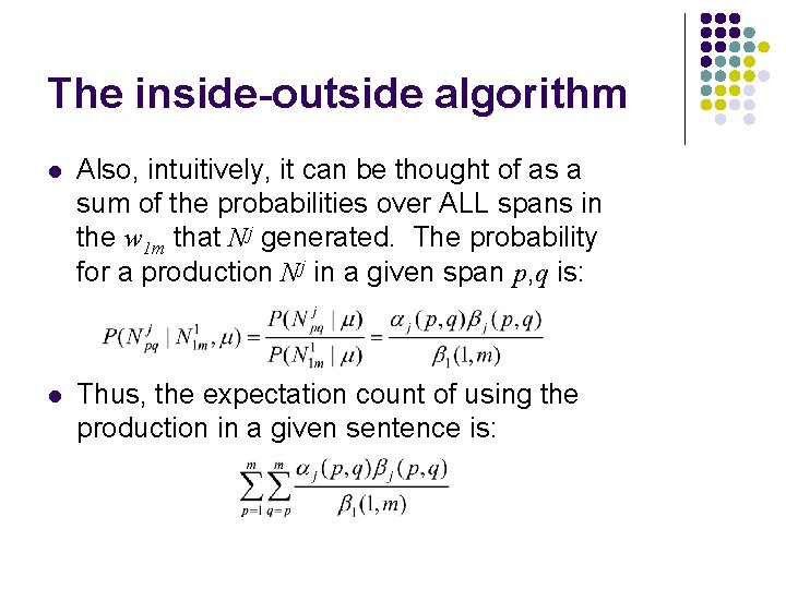
The inside-outside algorithm l What is the denominator l One possibility is to calculate the value of the numerator and sum the result over all non-terminals r, s. ?

The inside-outside algorithm l Also, intuitively, it can be thought of as a sum of the probabilities over ALL spans in the w 1 m that Nj generated. The probability for a production Nj in a given span p, q is: l Thus, the expectation count of using the production in a given sentence is:

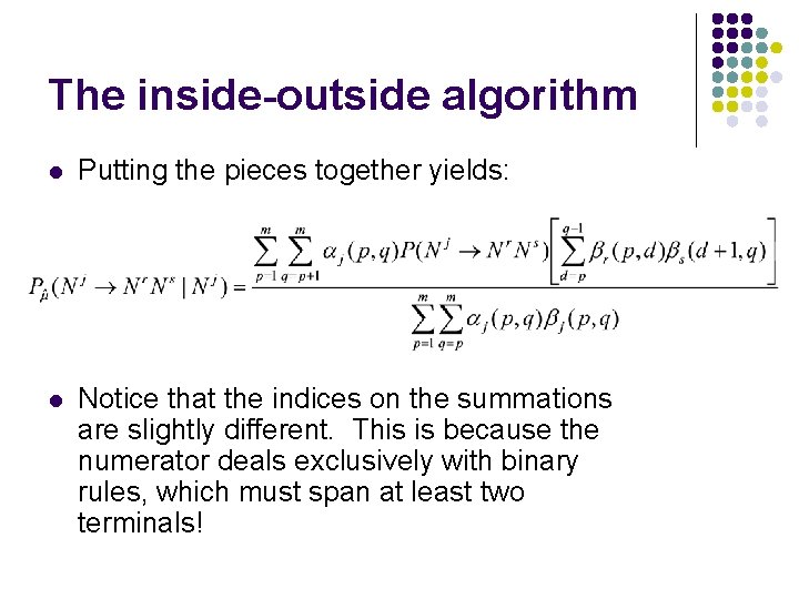
The inside-outside algorithm l Putting the pieces together yields: l Notice that the indices on the summations are slightly different. This is because the numerator deals exclusively with binary rules, which must span at least two terminals!