Numerical Relativistic Hydrodynamics Jos A Font Departamento de

Numerical Relativistic Hydrodynamics José A. Font Departamento de Astronomía y Astrofísica Universidad de Valencia (Spain) Lectures given at the School on “Structure and dynamics of compact objects”. Albert Einstein Institute, Golm (Germany). September 2004

Outline of the lectures • Introduction to the equations of (classical) fluid dynamics. • Conservation laws: general relativistic hydrodynamics equations. • Formulations of the general relativistic hydrodynamics equations (most used in numerical work): nonconservative vs conservative. • Nonlinear hyperbolic systems of conservation laws. • Riemann solvers and high-resolution shock-capturing (Godunov-type) schemes. • Example tests and applications in relativistic astrophysics. Bibliography: • A. J. Chorin & J. E. Marsden, “A mathematical introduction to fluid mechanics”, Springer Verlag (1990) • F. H. Shu, “The physics of astrophysics. Vol. II: Gas dynamics”, Mill Valley CA, University Science Books (1992) • R. J. Le. Veque, “Numerical methods for conservation laws”, Birkhäuser Verlag (1992) • E. F. Toro, “Riemann solvers and numerical methods for fluid dynamics: A practical introduction”, Springer Verlag (1999) • A. M. Anile, “Relativistic fluids and magneto-fluids”, Cambridge University Press (1989) • J. M. Martí & E. Müller, “Numerical hydrodynamics in special relativity”, Living Reviews in Relativity, 6, 7 (2003) • J. A. Font, “Numerical hydrodynamics in general relativity”, Living Reviews in Relativity, 6, 4, (2003) www. livingreviews. org

Astrophysical motivation General relativity and general relativistic hydrodynamics play a major role in the description of compact objects Core-collapse supernovae (neutron star formation) Gravitational collapse and black hole formation Coalescing binaries (NS/NS, BH/NS) Accretion on to black holes (jet formation, MRI of thick disks, etc) Nonlinear instabilities of rotating relativistic stars Time-dependent evolutions of fluid flow coupled to geometry is only possible through accurate, large-scale numerical simulations. Some scenarios can be described in the test-fluid approximation: hydrodynamical computations in (static) curved backgrounds (highly mature nowadays). Just as their classical counterparts, the GR hydrodynamic equations constitute a non-linear hyperbolic system. Solid mathematical foundations and accurate numerical methodology imported from CFD. A “preferred” choice: high-resolution shock-capturing schemes written in conservation form.

Fluid dynamics: introduction The defining property of fluids (liquids and gases) lies in the ease with which they may be deformed. A “simple fluid” (as opossed to a “simple solid”) might be defined as a material such that the relative positions of its constituent elements change by a large amount when suitable forces, however small in magnitude, are applied to the material. The gross properties of solids and fluids are directly related to their molecular structure and to the nature of the forces between the molecules. For most simple molecules, stable equilibrium between two molecules is achieved when their separation d 0 is of order 3 -4 x 10 -8 cm. The average spacing of the molecules in a gaseous phase at normal temperature and pressure is of the order of 10 d 0, while in liquids and solids is of the order of d 0. Fluid dynamics is concerned with the behaviour of matter in the large (average quantities per unit volume), on a macroscopic scale large compared with the distance between molecules, l>>d 0, not taking into account the molecular structure of fluids. Even when considering an infinitesimal volume element it must be assumed that it is much smaller than the dimensions of the fluid, L, but much larger than the distance between molecules, i. e. L>>l>>d 0. The macroscopic behaviour of fluids is furthermore supossed to be perfectly continuous in structure, and physical quantities such as mass, density, or momentum contained within a given small volume are regarded as being spread uniformly over that volume.

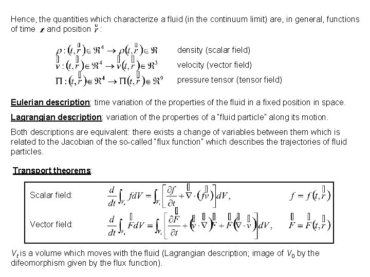
Hence, the quantities which characterize a fluid (in the continuum limit) are, in general, functions of time and position : density (scalar field) velocity (vector field) pressure tensor (tensor field) Eulerian description: time variation of the properties of the fluid in a fixed position in space. Lagrangian description: variation of the properties of a “fluid particle” along its motion. Both descriptions are equivalent: there exists a change of variables between them which is related to the Jacobian of the so-called “flux function” which describes the trajectories of fluid particles. Transport theorems: Scalar field: Vector field: Vt is a volume which moves with the fluid (Lagrangian description; image of V 0 by the difeomorphism given by the flux function).

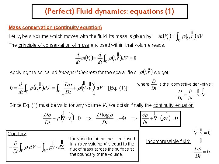
(Perfect) Fluid dynamics: equations (1) Mass conservation (continuity equation) Let Vt be a volume which moves with the fluid; its mass is given by The principle of conservation of mass enclosed within that volume reads: Applying the so-called transport theorem for the scalar field we get where is the “convective derivative”: Since Eq. (1) must be valid for any volume Vt, we obtain finally the continuity equation: Corolary: the variation of the mass enclosed in a fixed volume V is equal to the flux of mass across the surface at the boundary of the volume. Incompressible fluid:

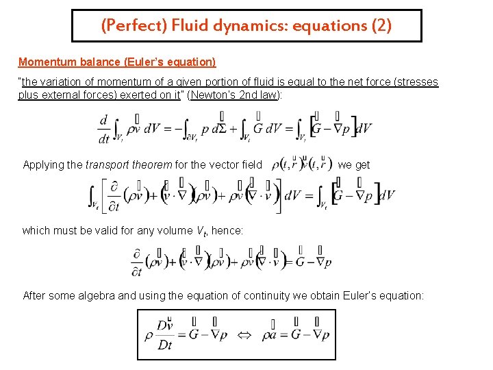
(Perfect) Fluid dynamics: equations (2) Momentum balance (Euler’s equation) “the variation of momentum of a given portion of fluid is equal to the net force (stresses plus external forces) exerted on it” (Newton’s 2 nd law): Applying the transport theorem for the vector field we get which must be valid for any volume Vt, hence: After some algebra and using the equation of continuity we obtain Euler’s equation:

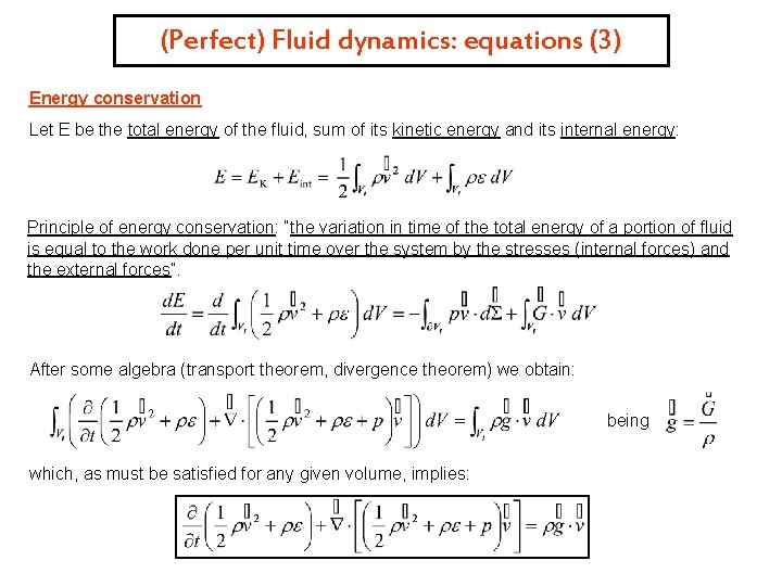
(Perfect) Fluid dynamics: equations (3) Energy conservation Let E be the total energy of the fluid, sum of its kinetic energy and its internal energy: Principle of energy conservation: “the variation in time of the total energy of a portion of fluid is equal to the work done per unit time over the system by the stresses (internal forces) and the external forces”. After some algebra (transport theorem, divergence theorem) we obtain: being which, as must be satisfied for any given volume, implies:

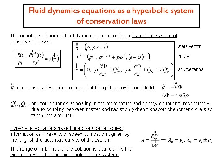
Fluid dynamics equations as a hyperbolic system of conservation laws The equations of perfect fluid dynamics are a nonlinear hyperbolic system of conservation laws: state vector fluxes source terms is a conservative external force field (e. g. the gravitational field): are source terms appearing in the momentum and energy equations, respectively, due to coupling between matter and radiation (when transport phenomena are also taken into account). Hyperbolic equations have finite propagation speed: information can travel with speed at most that given by the largest characteristic curves of the system. The range of influence of the solution is bounded by the eigenvalues of the Jacobian matrix of the system.

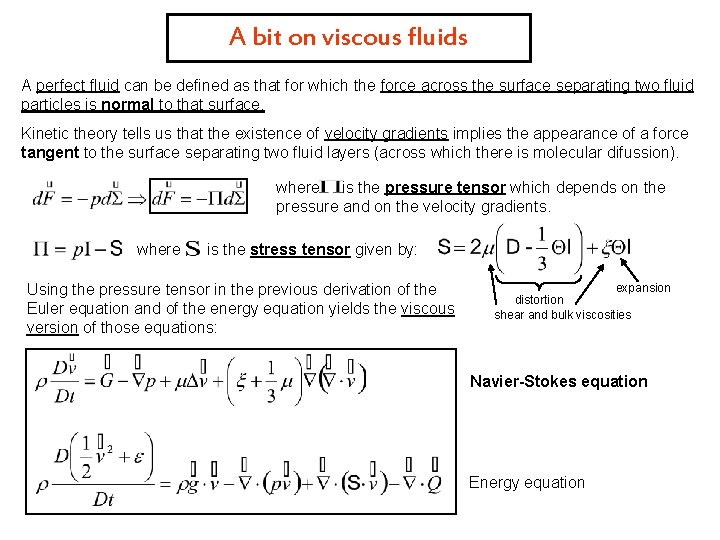
A bit on viscous fluids A perfect fluid can be defined as that for which the force across the surface separating two fluid particles is normal to that surface. Kinetic theory tells us that the existence of velocity gradients implies the appearance of a force tangent to the surface separating two fluid layers (across which there is molecular difussion). where is the pressure tensor which depends on the pressure and on the velocity gradients. where is the stress tensor given by: Using the pressure tensor in the previous derivation of the Euler equation and of the energy equation yields the viscous version of those equations: expansion distortion shear and bulk viscosities Navier-Stokes equation Energy equation

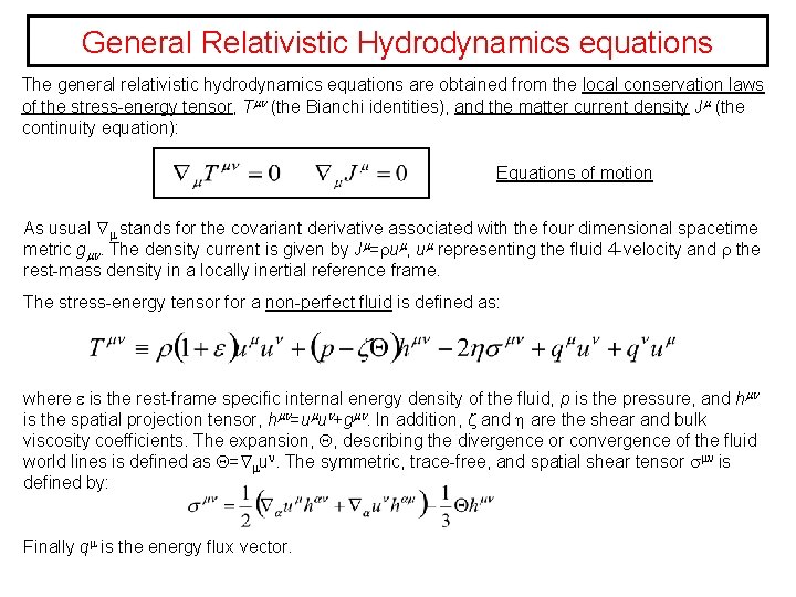
General Relativistic Hydrodynamics equations The general relativistic hydrodynamics equations are obtained from the local conservation laws of the stress-energy tensor, T (the Bianchi identities), and the matter current density J (the continuity equation): Equations of motion As usual stands for the covariant derivative associated with the four dimensional spacetime metric g . The density current is given by J = u , u representing the fluid 4 -velocity and the rest-mass density in a locally inertial reference frame. The stress-energy tensor for a non-perfect fluid is defined as: where is the rest-frame specific internal energy density of the fluid, p is the pressure, and h is the spatial projection tensor, h =u u +g . In addition, and are the shear and bulk viscosity coefficients. The expansion, , describing the divergence or convergence of the fluid world lines is defined as = u. The symmetric, trace-free, and spatial shear tensor is defined by: Finally q is the energy flux vector.

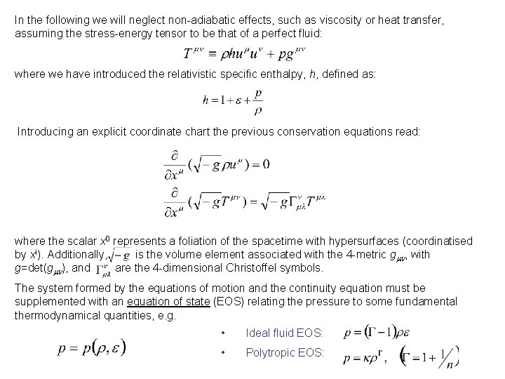
In the following we will neglect non-adiabatic effects, such as viscosity or heat transfer, assuming the stress-energy tensor to be that of a perfect fluid: where we have introduced the relativistic specific enthalpy, h, defined as: Introducing an explicit coordinate chart the previous conservation equations read: where the scalar x 0 represents a foliation of the spacetime with hypersurfaces (coordinatised by xi). Additionally, is the volume element associated with the 4 -metric g , with g=det(g ), and are the 4 -dimensional Christoffel symbols. The system formed by the equations of motion and the continuity equation must be supplemented with an equation of state (EOS) relating the pressure to some fundamental thermodynamical quantities, e. g. • Ideal fluid EOS: • Polytropic EOS:

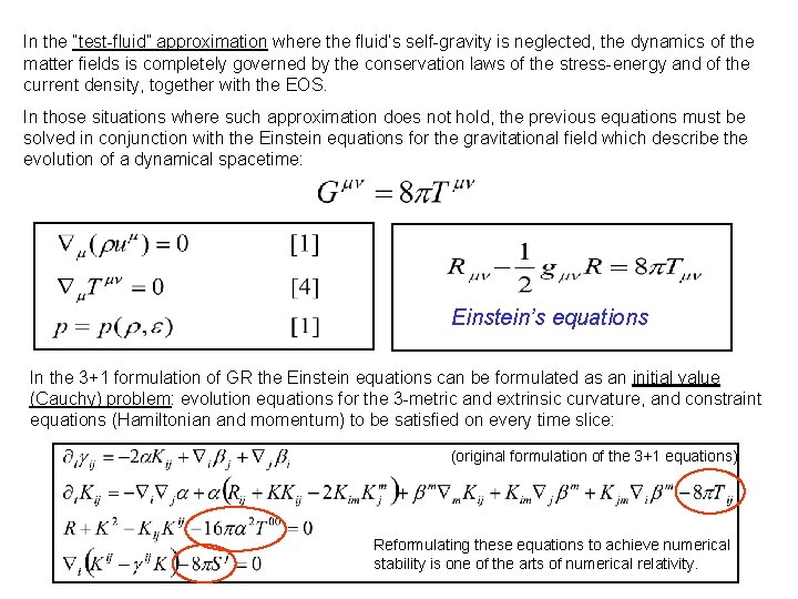
In the “test-fluid” approximation where the fluid’s self-gravity is neglected, the dynamics of the matter fields is completely governed by the conservation laws of the stress-energy and of the current density, together with the EOS. In those situations where such approximation does not hold, the previous equations must be solved in conjunction with the Einstein equations for the gravitational field which describe the evolution of a dynamical spacetime: Einstein’s equations In the 3+1 formulation of GR the Einstein equations can be formulated as an initial value (Cauchy) problem: evolution equations for the 3 -metric and extrinsic curvature, and constraint equations (Hamiltonian and momentum) to be satisfied on every time slice: (original formulation of the 3+1 equations) Reformulating these equations to achieve numerical stability is one of the arts of numerical relativity.

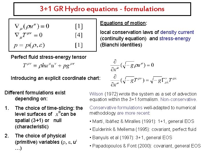
3+1 GR Hydro equations - formulations Equations of motion: local conservation laws of density current (continuity equation) and stress-energy (Bianchi identities) Perfect fluid stress-energy tensor Introducing an explicit coordinate chart: Different formulations exist depending on: Wilson (1972) wrote the system as a set of advection equation within the 3+1 formalism. Non-conservative. 1. The choice of time-slicing: the level surfaces of can be spatial (3+1) or null (characteristic) Conservative formulations well-adapted to numerical methodology are more recent: The choice of physical (primitive) variables ( , , ui …) • Banyuls et al (1997): 3+1, general EOS 2. • Martí, Ibáñez & Miralles (1991): 1+1, general EOS • Eulderink & Mellema (1995): covariant, perfect fluid • Papadopoulos & Font (2000): covariant, general EOS

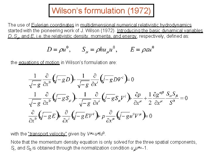
Wilson’s formulation (1972) The use of Eulerian coordinates in multidimensional numerical relativistic hydrodynamics started with the pioneering work of J. Wilson (1972). Introducing the basic dynamical variables D, S , and E, i. e. the relativistic density, momenta, and energy, respectively, defined as: the equations of motion in Wilson’s formulation are: with the “transport velocity” given by V =u /u 0. Note that the momentum density equation is only solved for the three spatial components, Si, and S 0 is obtained through the normalization condition u u =-1.

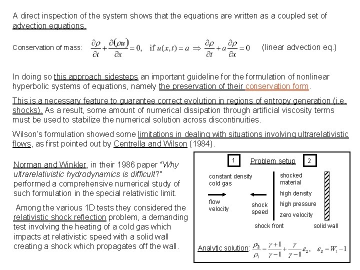
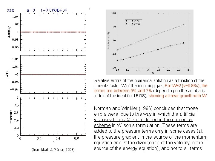
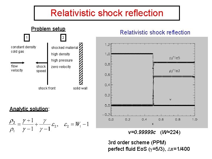
A direct inspection of the system shows that the equations are written as a coupled set of advection equations. (linear advection eq. ) Conservation of mass: In doing so this approach sidesteps an important guideline for the formulation of nonlinear hyperbolic systems of equations, namely the preservation of their conservation form. This is a necessary feature to guarantee correct evolution in regions of entropy generation (i. e. shocks). As a result, some amount of numerical dissipation through artificial viscosity terms must be used to stabilize the numerical solution across discontinuities. Wilson’s formulation showed some limitations in dealing with situations involving ultrarelativistic flows, as first pointed out by Centrella and Wilson (1984). Norman and Winkler, in their 1986 paper “Why ultrarelativistic hydrodynamics is difficult? ” performed a comprehensive numerical study of such formulation in the special relativistic limit. Among the various 1 D tests they considered the relativistic shock reflection problem, a demanding test involving the heating of a cold gas which impacts at relativistic speed with a solid wall creating a shock which propagates off the wall. 1 Problem setup 2 shocked material constant density cold gas high density flow velocity shock speed high pressure zero velocity shock front Analytic solution: solid wall

Relative errors of the numerical solution as a function of the Lorentz factor W of the incoming gas. For W≈2 (v≈0. 86 c), the errors are between 5% and 7% (depending on the adiabatic index of the ideal fluid EOS), showing a linear growth with W. (from Martí & Müller, 2003) Norman and Winkler (1986) concluded that those errors were due to the way in which the artificial viscosity terms Q are included in the numerical scheme in Wilson’s formulation. These terms are added to the pressure terms only in some cases (at the pressure gradient in the source of the momentum equation and at the divergence of the velocity in the source of the energy equation), and not to all terms.

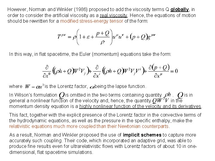
However, Norman and Winkler (1986) proposed to add the viscosity terms Q globally, in order to consider the artificial viscosity as a real viscosity. Hence, the equations of motion should be rewritten for a modified stress-energy tensor of the form: In this way, in flat spacetime, the Euler (momentum) equations take the form: where is the Lorentz factor, being the lapse function. In Wilson’s formulation is omitted in the two terms containing quantity. is in general a nonlinear function of the velocity and, hence, the quantity in the momentum density equation is a highly nonlinear function of the velocity and its derivatives. This fact, together with the explicit presence of the Lorentz factor in the convective terms of the hydrodynamic equations, as well as the pressure in the specific enthalpy, make the relativistic equations much more coupled than their Newtonian counterparts. As a result, Norman and Winkler proposed the use of implicit schemes to capture more accurately such coupling. Their code, which incorporated an adaptive grid, was able to produce fine results even for ultrarelativistic flows with Lorentz factors of about 10 in onedimensional, flat spacetime simulations.

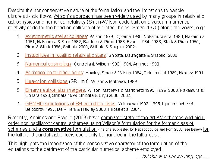
Despite the nonconservative nature of the formulation and the limitations to handle ultrarelativistic flows, Wilson’s approach has been widely used by many groups in relativistic astrophysics and numerical relativity (Smarr-Wilson code built on a vacuum numerical relativity code for the head-on collision of two black holes; Smarr 1975) along the years, e. g. : 1. Axisymmetric stellar collapse: Wilson 1979, Dykema 1980, Nakamura et al 1980, Nakamura 1981, Nakamura & Sato 1982, Bardeen & Piran 1983, Evans 1984, 1986, Stark & Piran 1985, Piran & Stark 1986, Shibata 2000, Shibata & Shapiro 2002. 2. Instabilities in rotating relativistic stars: Shibata, Baumgarte & Shapiro, 2000. 3. Numerical cosmology: Centrella & Wilson 1983, 1984, Anninos 1998. 4. Accretion on to black holes: Hawley, Smarr & Wilson 1984, Petrich et al 1989, Hawley 1991. 5. Heavy ion collisions (SR limit): Wilson & Mathews 1989. 6. Binary neutron star mergers: Wilson, Mathews & Marronetti 1995, 1996, 2000, Nakamura & Oohara 1998, Shibata 1999, Shibata & Uryu 2000, 2002. 7. GRMHD simulations of BH accretion disks: Yokosawa 1993, 1995, Igumenshchev & Belodorov 1997, De Villiers & Hawley 2003, Hirose et al 2004. Recently, Anninos and Fragile (2003) have compared state-of-the-art AV schemes and highorder non-oscillatory central schemes using Wilson’s formulation for the former class of schemes and a conservative formulation (the one suggested by Papadopoulos and Font 2000; see below) for the latter. Ultrarelativistic flows could only be handled in the latter case. This highlights the importance of the conservative character of the formulation of the equations to the detriment of the particular numerical scheme employed. … but this was known long ago …

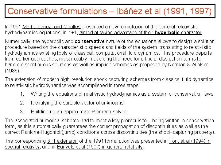
Conservative formulations – Ibáñez et al (1991, 1997) In 1991 Martí, Ibáñez, and Miralles presented a new formulation of the general relativistic hydrodynamics equations, in 1+1, aimed at taking advantage of their hyperbolic character. Numerically, the hyperbolic and conservative nature of the equations allows to design a solution procedure based on the characteristic speeds and fields of the system, translating to relativistic hydrodynamics existing tools of classical, computational fluid dynamics. This procedure departs from earlier approaches, most notably in avoiding the need for artificial dissipation terms to handle discontinuous solutions as well as implicit schemes as proposed by Norman & Winkler (1986). The extension of modern high-resolution shock-capturing schemes from classical fluid dynamics to relativistic hydrodynamics was accomplished in three steps: 1. Writing the equations of relativistic hydrodynamics as a system of conservation laws. 2. Identifying the suitable vector of unknowns. 3. Building up an approximate Riemann solver. The associated numerical scheme had to meet a key prerequisite – being written in conservation form, as this automatically guarantees the correct propagation of discontinuities as well as the correct Rankine-Hugoniot (jump) conditions across discontinuities (the shock-capturing property). The corresponding 3+1 extension of the 1991 formulation was presented in Font et al (1994) in special relativity, and in Banyuls et al (1997) in general relativity.

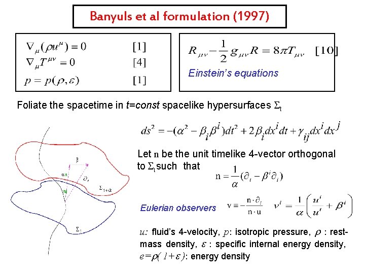
Banyuls et al formulation (1997) Einstein’s equations Foliate the spacetime in t=const spacelike hypersurfaces St Let n be the unit timelike 4 -vector orthogonal to St such that Eulerian observers u: fluid’s 4 -velocity, p: isotropic pressure, r : restmass density, e : specific internal energy density, e=r( 1+e ): energy density

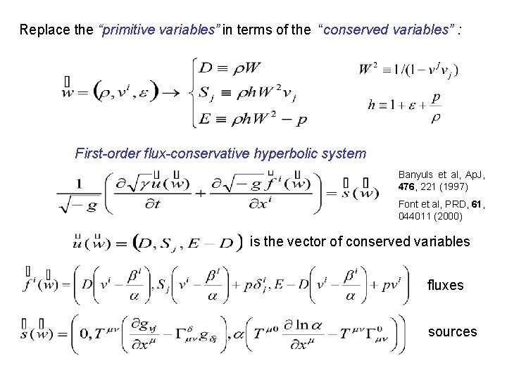
Replace the “primitive variables” in terms of the “conserved variables” : First-order flux-conservative hyperbolic system Banyuls et al, Ap. J, 476, 221 (1997) Font et al, PRD, 61, 044011 (2000) where is the vector of conserved variables fluxes sources

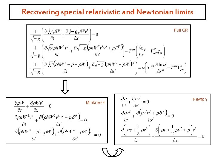
Recovering special relativistic and Newtonian limits Full GR Minkowski Newton

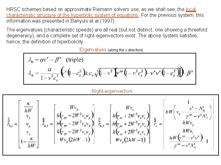
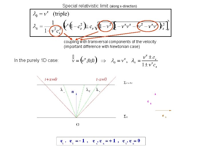
HRSC schemes based on approximate Riemann solvers use, as we shall see, the local characteristic structure of the hyperbolic system of equations. For the previous system, this information was presented in Banyuls et al (1997). The eigenvalues (characteristic speeds) are all real (but not distinct, one showing a threefold degeneracy), and a complete set of right-eigenvectors exist. The above system satisfies, hence, the definition of hiperbolicity. Eigenvalues (along the x direction) Right-eigenvectors

Special relativistic limit (along x-direction) coupling with transversal components of the velocity (important difference with Newtonian case) In the purely 1 D case:

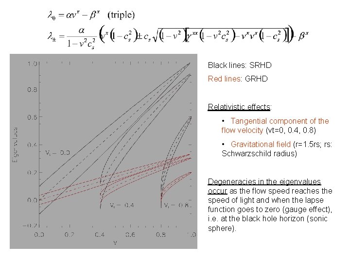
Black lines: SRHD Red lines: GRHD Relativistic effects: • Tangential component of the flow velocity (vt=0, 0. 4, 0. 8) • Gravitational field (r=1. 5 rs; rs: Schwarzschild radius) Degeneracies in the eigenvalues occur as the flow speed reaches the speed of light and when the lapse function goes to zero (gauge effect), i. e. at the black hole horizon (sonic sphere).

Existing applications of Banyuls et al formulation in relativistic astrophysics 1. Simulations of relativistic jets (SR): Martí et al 1994, 1995, 1997, Gómez et al 1995, 1997, 1998, Aloy et al 1999, 2003, Scheck et al 2002. GRB models: Aloy et al 2000, Aloy, Janka & Müller 2004. 3. Core collapse supernovae and GWs: Dimmelmeier, Font & Müller 2001, 2002 a, b, Dimmelmeier et al 2004, Cerdá-Durán et al 2004, Shibata & Sekiguchi 2004. QNM of rotating relativistic stars: Font, Stergioulas & Kokkotas 2000, Font et al 2001, 2002, Stergioulas & Font 2001, Stergioulas, Apostolatos & Font 2004, Shibata & Sekiguchi 2003. 5. Black hole formation: Baiotti et al 2004 (3 D whisky code). 6. Accretion on to black holes: Font & Ibáñez 1998 a, b, Font, Ibáñez & Papadopoulos 1999, Brandt et al 1998, Papadopoulos & Font 1998 a, b, Nagar et al 2004. 7. Disk accretion: Font & Daigne 2002 a, b, Daigne & Font 2004, Zanotti, Rezzolla & Font 2003, Rezzolla, Zanotti & Font 2003. 8. Binary neutron star mergers: Miller, Suen & Tobias 2001, Shibata, Taniguchi & Uryu 2003, Evans et al 2003, Miller, Gressman & Suen 2004.

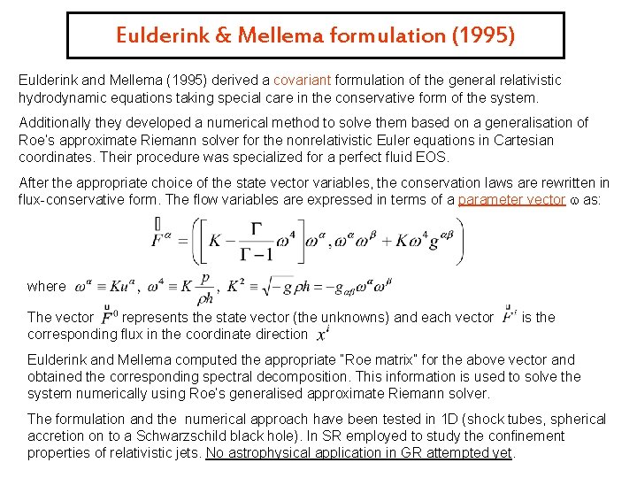
Eulderink & Mellema formulation (1995) Eulderink and Mellema (1995) derived a covariant formulation of the general relativistic hydrodynamic equations taking special care in the conservative form of the system. Additionally they developed a numerical method to solve them based on a generalisation of Roe’s approximate Riemann solver for the nonrelativistic Euler equations in Cartesian coordinates. Their procedure was specialized for a perfect fluid EOS. After the appropriate choice of the state vector variables, the conservation laws are rewritten in flux-conservative form. The flow variables are expressed in terms of a parameter vector as: where The vector represents the state vector (the unknowns) and each vector corresponding flux in the coordinate direction is the Eulderink and Mellema computed the appropriate “Roe matrix” for the above vector and obtained the corresponding spectral decomposition. This information is used to solve the system numerically using Roe’s generalised approximate Riemann solver. The formulation and the numerical approach have been tested in 1 D (shock tubes, spherical accretion on to a Schwarzschild black hole). In SR employed to study the confinement properties of relativistic jets. No astrophysical application in GR attempted yet.

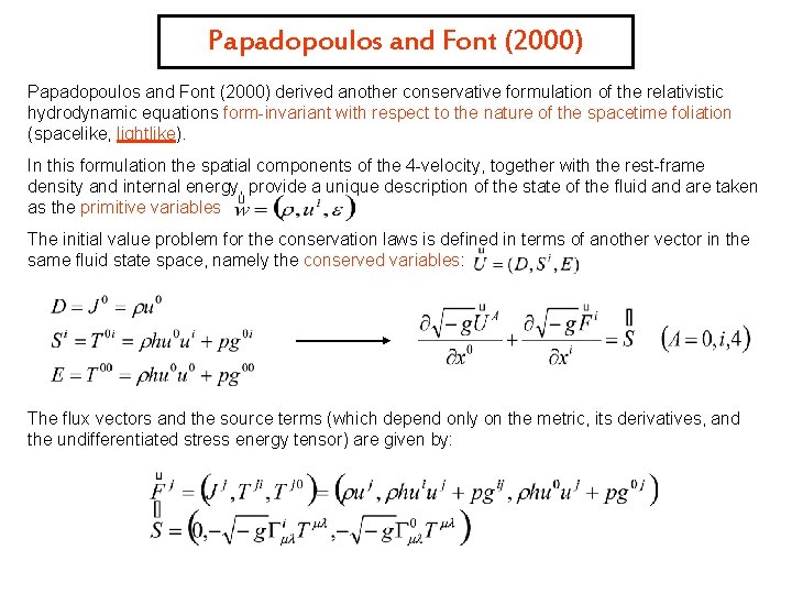
Papadopoulos and Font (2000) derived another conservative formulation of the relativistic hydrodynamic equations form-invariant with respect to the nature of the spacetime foliation (spacelike, lightlike). In this formulation the spatial components of the 4 -velocity, together with the rest-frame density and internal energy, provide a unique description of the state of the fluid and are taken as the primitive variables The initial value problem for the conservation laws is defined in terms of another vector in the same fluid state space, namely the conserved variables: The flux vectors and the source terms (which depend only on the metric, its derivatives, and the undifferentiated stress energy tensor) are given by:

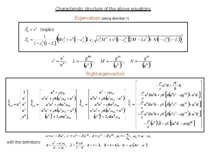
Characteristic structure of the above equations Eigenvalues (along direction 1) Right-eigenvectors with the definitions:

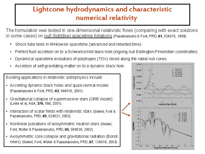
Lightcone hydrodynamics and characteristic numerical relativity The formulation was tested in one-dimensional relativistic flows (comparing with exact solutions in some cases) on null (lightlike) spacetime foliations (Papadopoulos & Font, PRD, 61, 024015, 1999): • Shock tube tests in Minkowski spacetime (advanced and retarded time). • Perfect fluid accretion on to a Schwarzschild black hole (ingoing null Eddington-Finkelstein coordinates). • Dynamical spacetime evolutions of polytropes (TOV) sliced along the radial null cones. • Accretion of self-gravitating matter on to a dynamic black hole. Existing applications in relativistic astrophysics include: • Accreting dynamic black holes and quasi-normal modes (Papadopoulos & Font, PRD, 63, 044016, 2001). • Gravitational collapse of supermassive stars (GRB model) (Linke et al, A&A, 376, 568, 2001). • Interaction of scalar fields with relativistic stars (Siebel, Font & Papadopoulos, PRD, 65, 024021, 2002). • Nonlinear pulsations of axisymmetric neutron stars (Siebel, Font, Müller & Papadopoulos, PRD, 65, 064038, 2002). • Axisymmetric core collapse and gravitational radiation (Bondi news) (Siebel, Font, Müller & Papadopoulos, PRD, 67, 124018, 2003).

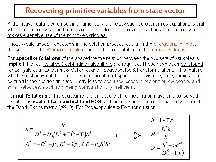
Recovering primitive variables from state vector A distinctive feature when solving numerically the relativistic hydrodynamics equations is that while the numerical algorithm updates the vector of conserved quantities, the numerical code makes extensive use of the primitive variables. Those would appear repeatedly in the solution procedure, e. g. in the characteristic fields, in the solution of the Riemann problem, and in the computation of the numerical fluxes. For spacelike foliations of the spacetime the relation between the two sets of variables is implicit. Hence, iterative (root-finding) algorithms are required. Those have been developed for Banyuls et al, Eulderink & Mellema, and Papadopoulos & Font formulations. This feature, which is distinctive of the equations of general (and special) relativistic hydrodynamics – not existing in the Newtonian case – may lead to accuracy losses in regions of low density and small velocities, apart from being computationally inefficient. For null foliations of the spacetime, the procedure of connecting primitive and conserved variables is explicit for a perfect fluid EOS, a direct consequence of the particular form of the Bondi-Sachs metric (g 00=0). For Papadopoulos & Font formulation:

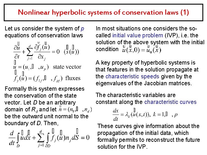
Nonlinear hyperbolic systems of conservation laws (1) Let us consider the system of p equations of conservation laws Formally this system expresses the conservation of the state vector. Let D be an arbitrary domain of Rd and let be the outward unit normal to the boundary of D. Then, In most situations one considers the socalled initial value problem (IVP), i. e. the solution of the above system with the initial condition A key property of hyperbolic systems is that features in the solution propagate at the characteristic speeds given by the eigenvalues of the Jacobian matrices. The characteristic variables are constant along the characteristic curves These curves give information about the propagation of the initial data, which formally permits to reconstruct the future solution for the IVP.

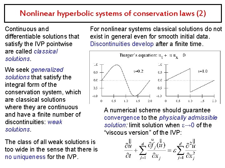
Nonlinear hyperbolic systems of conservation laws (2) Continuous and differentiable solutions that satisfy the IVP pointwise are called classical solutions. For nonlinear systems classical solutions do not exist in general even for smooth initial data. Discontinuities develop after a finite time. We seek generalized solutions that satisfy the integral form of the conservation system, which are classical solutions where they are continuous and have a finite number of discontinuities: weak solutions. The class of all weak solutions is too wide in the sense that there is no uniqueness for the IVP. A numerical scheme should guarantee convergence to the physically admissible solution: limit solution when → 0 of the “viscous version” of the IVP:

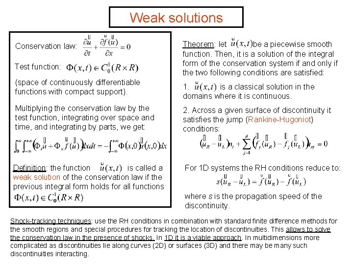
Weak solutions Conservation law: Test function: (space of continuously differentiable functions with compact support). Theorem: let be a piecewise smooth function. Then, it is a solution of the integral form of the conservation system if and only if the two following conditions are satisfied: 1. is a classical solution in the domains where it is continuous. Multiplying the conservation law by the test function, integrating over space and time, and integrating by parts, we get: 2. Across a given surface of discontinuity it satisfies the jump (Rankine-Hugoniot) conditions: Definition: the function is called a weak solution of the conservation law if the previous integral form holds for all functions For 1 D systems the RH conditions reduce to: where s is the propagation speed of the discontinuity. Shock-tracking techniques: use the RH conditions in combination with standard finite difference methods for the smooth regions and special procedures for tracking the location of discontinuities. This allows to solve the conservation law in the presence of shocks. In 1 D it is a viable approach. In multidimensions more complicated as discontinuities lie along curves (2 D) or surfaces (3 D) and there may be many such discontinuities interacting.

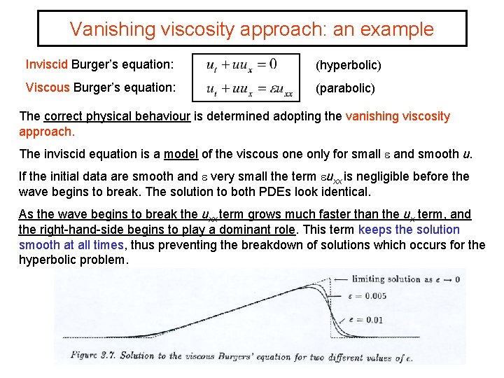
Vanishing viscosity approach: an example Inviscid Burger’s equation: (hyperbolic) Viscous Burger’s equation: (parabolic) The correct physical behaviour is determined adopting the vanishing viscosity approach. The inviscid equation is a model of the viscous one only for small and smooth u. If the initial data are smooth and very small the term uxx is negligible before the wave begins to break. The solution to both PDEs look identical. As the wave begins to break the uxx term grows much faster than the ux term, and the right-hand-side begins to play a dominant role. This term keeps the solution smooth at all times, thus preventing the breakdown of solutions which occurs for the hyperbolic problem.

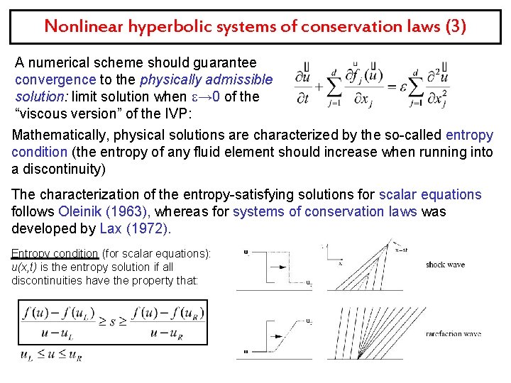
Nonlinear hyperbolic systems of conservation laws (3) A numerical scheme should guarantee convergence to the physically admissible solution: limit solution when → 0 of the “viscous version” of the IVP: Mathematically, physical solutions are characterized by the so-called entropy condition (the entropy of any fluid element should increase when running into a discontinuity) The characterization of the entropy-satisfying solutions for scalar equations follows Oleinik (1963), whereas for systems of conservation laws was developed by Lax (1972). Entropy condition (for scalar equations): u(x, t) is the entropy solution if all discontinuities have the property that:

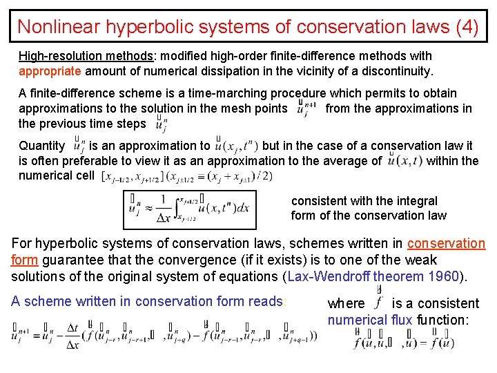
Nonlinear hyperbolic systems of conservation laws (4) High-resolution methods: modified high-order finite-difference methods with appropriate amount of numerical dissipation in the vicinity of a discontinuity. A finite-difference scheme is a time-marching procedure which permits to obtain approximations to the solution in the mesh points from the approximations in the previous time steps Quantity is an approximation to but in the case of a conservation law it is often preferable to view it as an approximation to the average of within the numerical cell consistent with the integral form of the conservation law For hyperbolic systems of conservation laws, schemes written in conservation form guarantee that the convergence (if it exists) is to one of the weak solutions of the original system of equations (Lax-Wendroff theorem 1960). A scheme written in conservation form reads: where is a consistent numerical flux function:

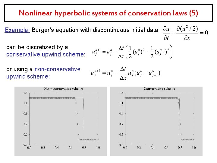
Nonlinear hyperbolic systems of conservation laws (5) Example: Burger’s equation with discontinuous initial data can be discretized by a conservative upwind scheme: or using a non-conservative upwind scheme:

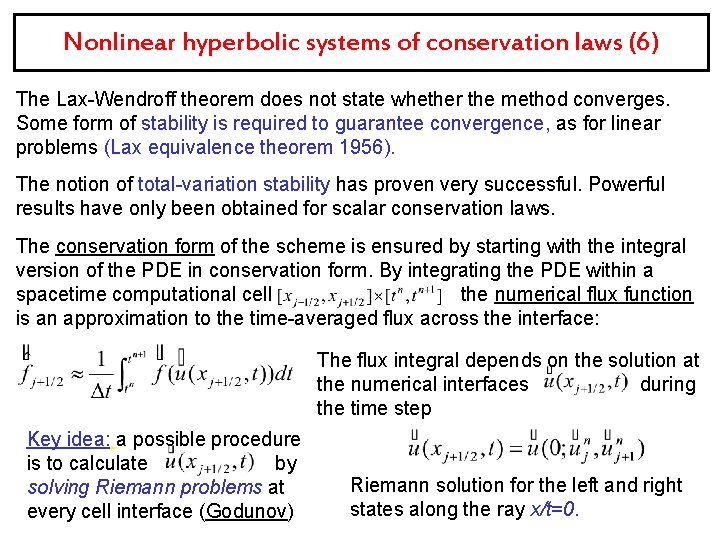
Nonlinear hyperbolic systems of conservation laws (6) The Lax-Wendroff theorem does not state whether the method converges. Some form of stability is required to guarantee convergence, as for linear problems (Lax equivalence theorem 1956). The notion of total-variation stability has proven very successful. Powerful results have only been obtained for scalar conservation laws. The conservation form of the scheme is ensured by starting with the integral version of the PDE in conservation form. By integrating the PDE within a spacetime computational cell the numerical flux function is an approximation to the time-averaged flux across the interface: The flux integral depends on the solution at the numerical interfaces during the time step Key idea: a possible procedure is to calculate by solving Riemann problems at every cell interface (Godunov) Riemann solution for the left and right states along the ray x/t=0.

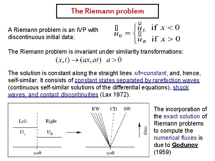
The Riemann problem A Riemann problem is an IVP with discontinuous initial data: The Riemann problem is invariant under similarity transformations: The solution is constant along the straight lines x/t=constant, and, hence, self-similar. It consists of constant states separated by rarefaction waves (continuous self-similar solutions of the differential equations), shock waves, and contact discontinuities (Lax 1972). The incorporation of the exact solution of Riemann problems to compute the numerical fluxes is due to Godunov (1959)

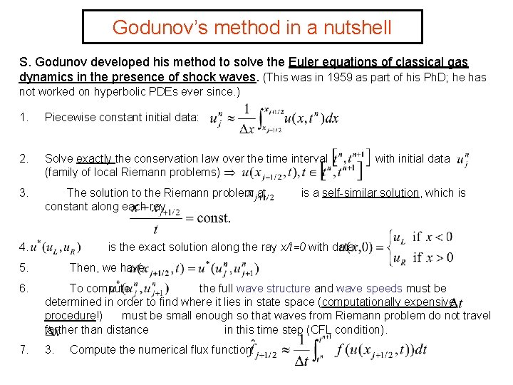
Godunov’s method in a nutshell S. Godunov developed his method to solve the Euler equations of classical gas dynamics in the presence of shock waves. (This was in 1959 as part of his Ph. D; he has not worked on hyperbolic PDEs ever since. ) 1. Piecewise constant initial data: 2. Solve exactly the conservation law over the time interval (family of local Riemann problems) 3. The solution to the Riemann problem at constant along each ray 4. with initial data is a self-similar solution, which is is the exact solution along the ray x/t=0 with data: 5. Then, we have 6. To compute the full wave structure and wave speeds must be determined in order to find where it lies in state space (computationally expensive procedure!) must be small enough so that waves from Riemann problem do not travel farther than distance in this time step (CFL condition). 7. 3. Compute the numerical flux function:

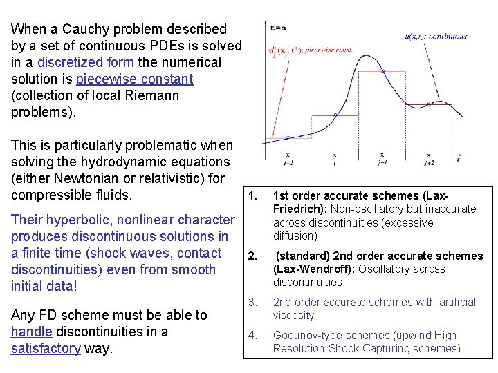
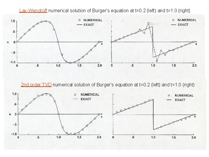
When a Cauchy problem described by a set of continuous PDEs is solved in a discretized form the numerical solution is piecewise constant (collection of local Riemann problems). This is particularly problematic when solving the hydrodynamic equations (either Newtonian or relativistic) for compressible fluids. 1. Their hyperbolic, nonlinear character produces discontinuous solutions in a finite time (shock waves, contact 2. discontinuities) even from smooth initial data! Any FD scheme must be able to handle discontinuities in a satisfactory way. 1 st order accurate schemes (Lax. Friedrich): Non-oscillatory but inaccurate across discontinuities (excessive diffusion) (standard) 2 nd order accurate schemes (Lax-Wendroff): Oscillatory across discontinuities 3. 2 nd order accurate schemes with artificial viscosity 4. Godunov-type schemes (upwind High Resolution Shock Capturing schemes)

Lax-Wendroff numerical solution of Burger’s equation at t=0. 2 (left) and t=1. 0 (right) 2 nd order TVD numerical solution of Burger’s equation at t=0. 2 (left) and t=1. 0 (right)

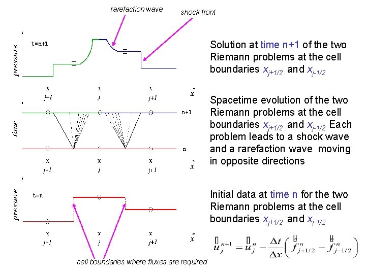
rarefaction wave shock front Solution at time n+1 of the two Riemann problems at the cell boundaries xj+1/2 and xj-1/2 Spacetime evolution of the two Riemann problems at the cell boundaries xj+1/2 and xj-1/2. Each problem leads to a shock wave and a rarefaction wave moving in opposite directions Initial data at time n for the two Riemann problems at the cell boundaries xj+1/2 and xj-1/2 cell boundaries where fluxes are required

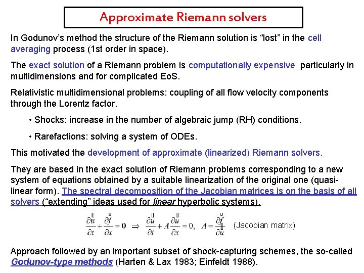
Approximate Riemann solvers In Godunov’s method the structure of the Riemann solution is “lost” in the cell averaging process (1 st order in space). The exact solution of a Riemann problem is computationally expensive, particularly in multidimensions and for complicated Eo. S. Relativistic multidimensional problems: coupling of all flow velocity components through the Lorentz factor. • Shocks: increase in the number of algebraic jump (RH) conditions. • Rarefactions: solving a system of ODEs. This motivated the development of approximate (linearized) Riemann solvers. They are based in the exact solution of Riemann problems corresponding to a new system of equations obtained by a suitable linearization of the original one (quasilinear form). The spectral decomposition of the Jacobian matrices is on the basis of all solvers (“extending” ideas used for linear hyperbolic systems). (Jacobian matrix) Approach followed by an important subset of shock-capturing schemes, the so-called Godunov-type methods (Harten & Lax 1983; Einfeldt 1988).

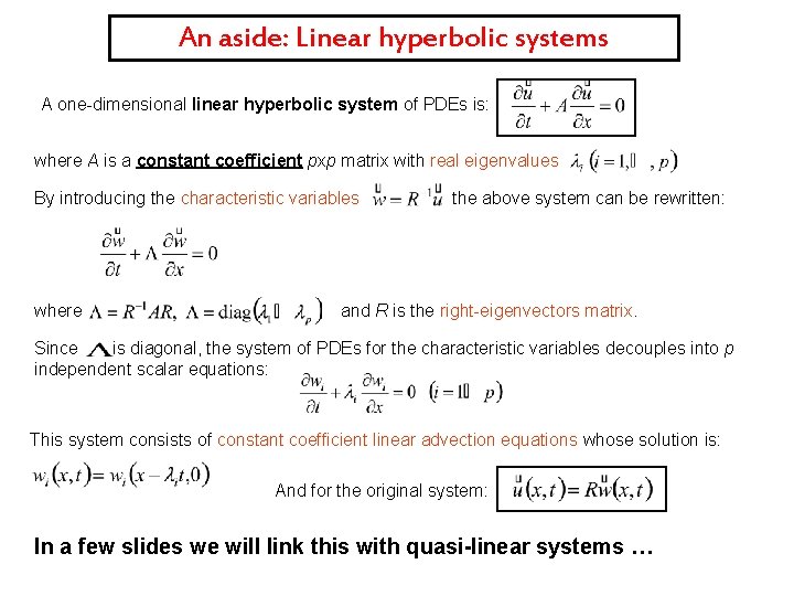
An aside: Linear hyperbolic systems A one-dimensional linear hyperbolic system of PDEs is: where A is a constant coefficient pxp matrix with real eigenvalues By introducing the characteristic variables where the above system can be rewritten: and R is the right-eigenvectors matrix. Since is diagonal, the system of PDEs for the characteristic variables decouples into p independent scalar equations: This system consists of constant coefficient linear advection equations whose solution is: And for the original system: In a few slides we will link this with quasi-linear systems …

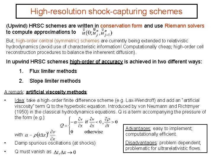
High-resolution shock-capturing schemes (Upwind) HRSC schemes are written in conservation form and use Riemann solvers to compute approximations to But, high-order central (symmetric) schemes are currently being extended to relativistic hydrodynamics (avoid use of characteristic information! Computationally cheap; high-order cell reconstruction procedures to balance the inhererent diffusion). In upwind HRSC schemes high-order of accuracy is achieved in two different ways: 1. Flux limiter methods 2. Slope limiter methods A remark: artificial viscosity methods: • Idea: take a high-order finite difference scheme (e. g. Lax-Wendroff) and add an “artificial viscosity” term Q to the hyperbolic equation. Introduced by von Neumann and Richtmyer (1950) in the classical hydrodynamics equations. Q is a term accompanying the pressure of the form (e. g. ): with • Damp spurious oscillations (at shocks) • Q must vanish as Advantages: easy to implement; computationally efficient. Disadvantages: problem dependent; problematic for ultrarelativistic flows.

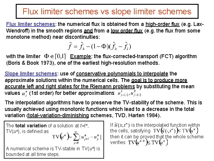
Flux limiter schemes vs slope limiter schemes Flux limiter schemes: the numerical flux is obtained from a high-order flux (e. g. Lax. Wendroff) in the smooth regions and from a low order flux (e. g. the flux from some monotone method) near discontinuities: with the limiter Example: the flux-corrected-transport (FCT) algorithm (Boris & Book 1973), one of the earliest high-resolution methods. Slope limiter schemes: use of conservative polynomials to interpolate the approximate solutions within the numerical cells. The goal is to produce more accurate left and right states for the Riemann problems by substituting the mean values (1 st order) for better approximations The interpolation algorithms have to preserve the TV-stability of the scheme. This is usually achieved using monotonic functions which lead to a decrease in the total variation (total-variation-diminishing schemes, TVD, Harten 1984). The total variation of a solution at t=tn, TV(un), is defined as A numerical scheme is TV-stable in TV(un) is bounded at all time steps. If is the interpolated function within the cells, satisfying then it can be proved that the whole scheme verifies

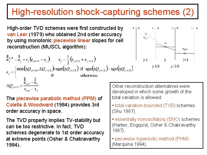
High-resolution shock-capturing schemes (2) High-order TVD schemes were first constructed by van Leer (1979) who obtained 2 nd order accuracy by using monotonic piecewise linear slopes for cell reconstruction (MUSCL algorithm): The piecewise parabolic method (PPM) of Colella & Woodward (1984) provides 3 rd order accuracy in space. The TVD property implies TV-stability but can be too restrictive. In fact, TVD schemes degenerate to 1 st order accuracy at extreme points (Osher & Chakravarthy 1984). Other reconstruction alternatives were developed in which some growth of the total variation is allowed: • total-variation-bounded (TVB) schemes (Shu 1987). • essentially nonoscillatory (ENO) schemes (Harten, Engquist, Osher & Chakravarthy 1987). • piecewise hyperbolic method (PHM) (Marquina 1994).

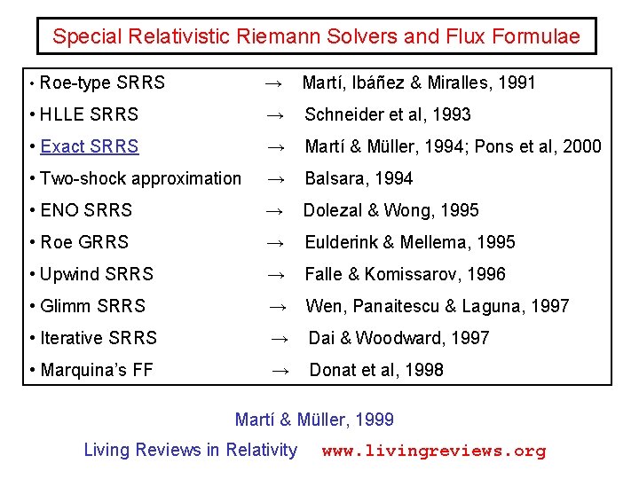
Special Relativistic Riemann Solvers and Flux Formulae • Roe-type SRRS → Martí, Ibáñez & Miralles, 1991 • HLLE SRRS → Schneider et al, 1993 • Exact SRRS → Martí & Müller, 1994; Pons et al, 2000 • Two-shock approximation → Balsara, 1994 • ENO SRRS → Dolezal & Wong, 1995 • Roe GRRS → Eulderink & Mellema, 1995 • Upwind SRRS → Falle & Komissarov, 1996 • Glimm SRRS → Wen, Panaitescu & Laguna, 1997 • Iterative SRRS → Dai & Woodward, 1997 • Marquina’s FF → Donat et al, 1998 Martí & Müller, 1999 Living Reviews in Relativity www. livingreviews. org

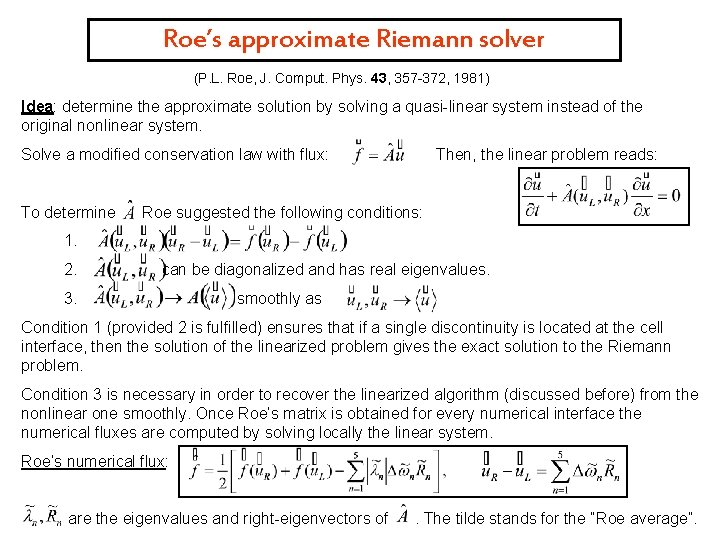
Roe’s approximate Riemann solver (P. L. Roe, J. Comput. Phys. 43, 357 -372, 1981) Idea: determine the approximate solution by solving a quasi-linear system instead of the original nonlinear system. Solve a modified conservation law with flux: To determine Then, the linear problem reads: Roe suggested the following conditions: 1. 2. can be diagonalized and has real eigenvalues. 3. smoothly as Condition 1 (provided 2 is fulfilled) ensures that if a single discontinuity is located at the cell interface, then the solution of the linearized problem gives the exact solution to the Riemann problem. Condition 3 is necessary in order to recover the linearized algorithm (discussed before) from the nonlinear one smoothly. Once Roe’s matrix is obtained for every numerical interface the numerical fluxes are computed by solving locally the linear system. Roe’s numerical flux: are the eigenvalues and right-eigenvectors of . The tilde stands for the “Roe average”.

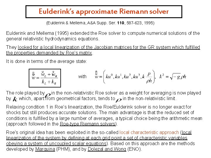
Eulderink’s approximate Riemann solver (Eulderink & Mellema, A&A Supp. Ser. 110, 587 -623, 1995) Eulderink and Mellema (1995) extended the Roe solver to compute numerical solutions of the general relativistic hydrodynamics equations. They looked for a local linearization of the Jacobian matrices for the GR system which fulfilled the properties demanded by Roe’s matrix. It is done in terms of the average state: with The role played by in the non-relativistic Roe solver as a weight for averaging is now played by which, apart from geometrical factors, tends to in the non-relativistic limit. Relaxing condition 1 in Roe’s linearization, the Roe/Eulderink solver is no longer exact for shocks but still produces accurate solutions. The main advantage is that the reduced set of conditions is fulfilled by a large number of averages, a typical choice being the arithmetic mean (approach followed in the Roe-type Riemann solvers). Roe’s original idea has been exploited in the so-called local characteristic approach (local linearization of the system by defining at each grid point a set of characteristic variables obeying a system of uncoupled scalar equations). Based on this approach are the methods developed by Marquina (PHM), and by Dolezal and Wong (ENO).

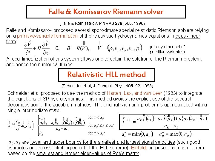
Falle & Komissarov Riemann solver (Falle & Komissarov, MNRAS 278, 586, 1996) Falle and Komissarov proposed several approximate special relativistic Riemann solvers relying on a primitive-variable formulation of the relativistic hydrodynamics equations in quasi-linear form: (or any other set of primitive variables) A local limearization of this system allows one to obtain the solution of the Riemann problem, and hence the numerical fluxes. Relativistic HLL method (Schneider et al, J. Comput. Phys. 105, 92, 1993) Schneider et al proposed to use the method of Harten, Lax, and van Leer (1983) to integrate the equations of SR hydrodynamics. This method avoids the explicit use of the spectral decomposition of the Jacobian matrices. The original Riemann problem is approximated with a single intermediate state: are lower and upper bounds for the smallest and largest signal velocities (such good estimates are an essential ingredient of the HLL scheme). Einfeldt proposed calculating them based on the smallest and largest eigenvalues of Roe’s matrix.

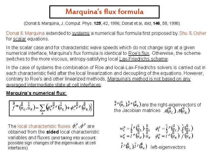
Marquina’s flux formula (Donat & Marquina, J. Comput. Phys. 125, 42, 1996; Donat et al, ibid, 146, 58, 1998) Donat & Marquina extended to systems a numerical flux formula first proposed by Shu & Osher for scalar equations. In the scalar case and for characteristic wave speeds which do not change sign at a given numerical interface, Marquina’s flux formula is identical to Roe’s flux. Otherwise, the scheme switches to the more viscous, entropy-satisfying local Lax-Friedrichs scheme. In the case of systems the combination of Roe and local-Lax-Friedrichs solvers is carried out in each characteristic field after the local linearization and decoupling of the equations. However, contrary to Roe’s and other linearized methods, Marquina’s method is not based on any averaged intermediate state at cell interfaces. Marquina’s numerical flux: are the right-eigenvectors of the Jacobian matrices The local characteristic fluxes are obtained from the sided local characteristic variables and fluxes (and taking into account possible sign changes of the eigenvalues at cell interfaces). left-eigenvectors

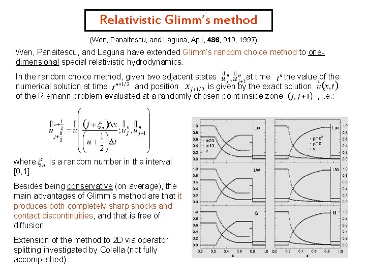
Relativistic Glimm’s method (Wen, Panaitescu, and Laguna, Ap. J, 486, 919, 1997) Wen, Panaitescu, and Laguna have extended Glimm’s random choice method to onedimensional special relativistic hydrodynamics. In the random choice method, given two adjacent states at time the value of the numerical solution at time and position is given by the exact solution of the Riemann problem evaluated at a randomly chosen point inside zone , i. e. : where [0, 1]. is a random number in the interval Besides being conservative (on average), the main advantages of Glimm’s method are that it produces both completely sharp shocks and contact discontinuities, and that is free of diffusion. Extension of the method to 2 D via operator splitting investigated by Colella (not fully accomplished).

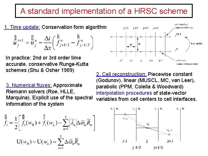
A standard implementation of a HRSC scheme 1. Time update: Conservation form algorithm In practice: 2 nd or 3 rd order time accurate, conservative Runge-Kutta schemes (Shu & Osher 1989) 2. Cell reconstruction: Piecewise constant (Godunov), linear (MUSCL, MC, van Leer), 3. Numerical fluxes: Approximate parabolic (PPM, Colella & Woodward) Riemann solvers (Roe, HLLE, interpolation procedures of state-vector Marquina). Explicit use of the spectral variables from cell centers to cell interfaces. information of the system

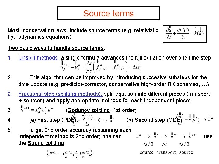
Source terms Most “conservation laws” include source terms (e. g. relativistic hydrodynamics equations) Two basic ways to handle source terms: 1. Unsplit methods: a single formula advances the full equation over one time step 2. This algorithm can be improved by introducing succesive substeps for the time update (e. g. predictor-corrector, conservative high-order RK schemes, …) 2. Fractional step (splitting methods): split equation into different pieces (transport + sources) and apply appropriate methods for each independent piece: 3. 4. 5. (Godunov splitting, 1 st order) (a) First step (PDE): (b) Second step (ODE): to get 2 nd order accuracy (assuming each independent method is 2 nd order) one can the Strang splitting: use

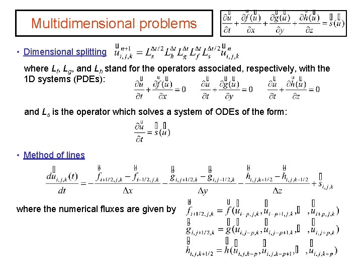
Multidimensional problems • Dimensional splitting where Lf, Lg, and Lh stand for the operators associated, respectively, with the 1 D systems (PDEs): and Ls is the operator which solves a system of ODEs of the form: • Method of lines where the numerical fluxes are given by

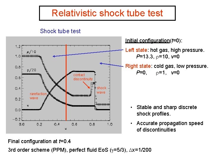
Relativistic shock tube test Shock tube test Initial configuration(t=0): Left state: hot gas, high pressure. P=13. 3, =10, v=0 Right state: cold gas, low pressure. P=0, =1, v=0 contact discontinuity rarefaction wave shock wave • Stable and sharp discrete shock profiles. • Accurate propagation speed of discontinuities Final configuration at t=0. 4 3 rd order scheme (PPM), perfect fluid Eo. S ( =5/3), x=1/200

Relativistic shock reflection Problem setup 1 Relativistic shock reflection 2 constant density cold gas shocked material high density high pressure flow velocity shock speed zero velocity shock front solid wall Analytic solution: v=0. 99999 c (W=224) 3 rd order scheme (PPM) perfect fluid Eo. S ( =5/3), x=1/400

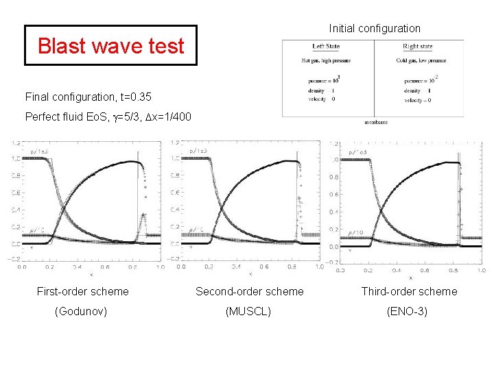
Initial configuration Blast wave test Final configuration, t=0. 35 Perfect fluid Eo. S, =5/3, x=1/400 First-order scheme Second-order scheme Third-order scheme (Godunov) (MUSCL) (ENO-3)

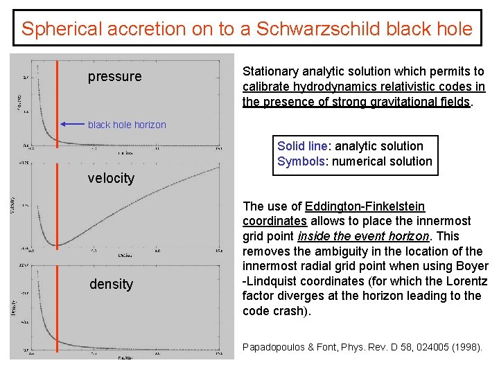
Spherical accretion on to a Schwarzschild black hole pressure Stationary analytic solution which permits to calibrate hydrodynamics relativistic codes in the presence of strong gravitational fields. black hole horizon Solid line: analytic solution Symbols: numerical solution velocity density The use of Eddington-Finkelstein coordinates allows to place the innermost grid point inside the event horizon. This removes the ambiguity in the location of the innermost radial grid point when using Boyer -Lindquist coordinates (for which the Lorentz factor diverges at the horizon leading to the code crash). Papadopoulos & Font, Phys. Rev. D 58, 024005 (1998).

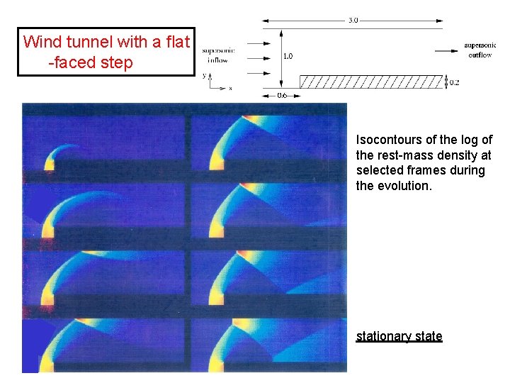
Wind tunnel with a flat -faced step Isocontours of the log of the rest-mass density at selected frames during the evolution. stationary state

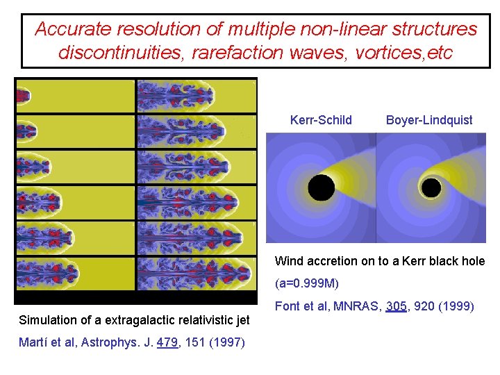
Accurate resolution of multiple non-linear structures discontinuities, rarefaction waves, vortices, etc Kerr-Schild Boyer-Lindquist Wind accretion on to a Kerr black hole (a=0. 999 M) Font et al, MNRAS, 305, 920 (1999) Simulation of a extragalactic relativistic jet Martí et al, Astrophys. J. 479, 151 (1997)

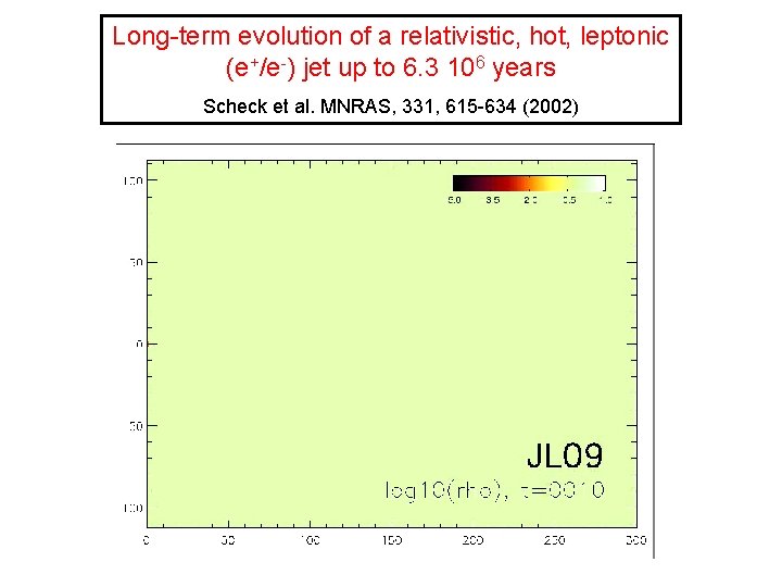
Long-term evolution of a relativistic, hot, leptonic (e+/e-) jet up to 6. 3 106 years Scheck et al. MNRAS, 331, 615 -634 (2002)

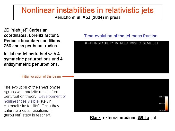
Nonlinear instabilities in relativistic jets Perucho et al, Ap. J (2004) in press 2 D “slab jet” Cartesian coordinates. Lorentz factor 5. Periodic boundary conditions. 256 zones per beam radius. Time evolution of the jet mass fraction Initial model perturbed with 4 symmetric perturbations and 4 antisymmetric perturbations. Initial location of the beam The evolution of the linear phase agrees with analytic results from perturbation theory. Development of nonlinearities visible (Kelvin. Helmholtz instability). Once they saturate a quasi-equilibrium (turbulent) state is reached. Black: external medium. White: jet

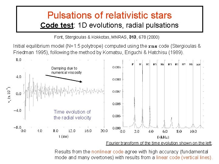
Pulsations of relativistic stars Code test: 1 D evolutions, radial pulsations Font, Stergioulas & Kokkotas, MNRAS, 313, 678 (2000) Initial equilibrium model (N=1. 5 polytrope) computed using the rns code (Stergioulas & Friedman 1995), following the method by Komatsu, Eriguchi & Hatchisu (1989). Damping due to numerical viscosity Time evolution of the radial velocity Fourier transform of the time evolution shown on the left. Results from the nonlinear code agree with high accuracy (fundamental mode and many overtones) with results from a linear code (vertical lines).

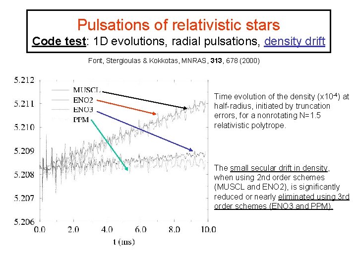
Pulsations of relativistic stars Code test: 1 D evolutions, radial pulsations, density drift Font, Stergioulas & Kokkotas, MNRAS, 313, 678 (2000) Time evolution of the density (x 10 -4) at half-radius, initiated by truncation errors, for a nonrotating N=1. 5 relativistic polytrope. The small secular drift in density, when using 2 nd order schemes (MUSCL and ENO 2), is significantly reduced or nearly eliminated using 3 rd order schemes (ENO 3 and PPM).

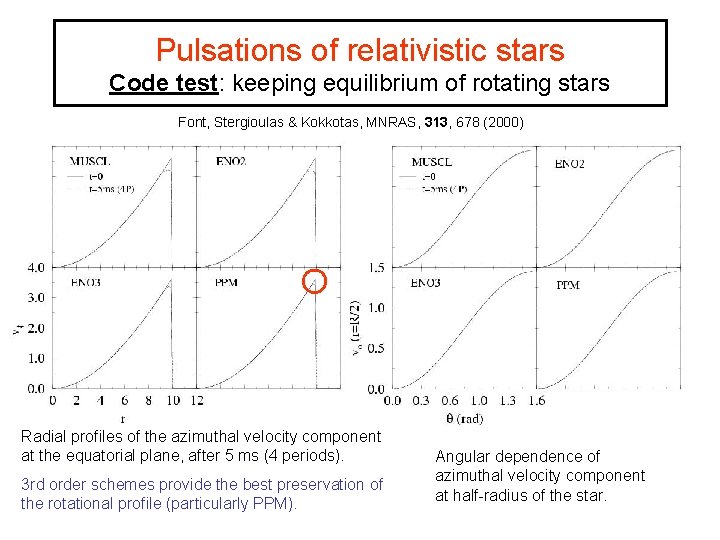
Pulsations of relativistic stars Code test: keeping equilibrium of rotating stars Font, Stergioulas & Kokkotas, MNRAS, 313, 678 (2000) Radial profiles of the azimuthal velocity component at the equatorial plane, after 5 ms (4 periods). 3 rd order schemes provide the best preservation of the rotational profile (particularly PPM). Angular dependence of azimuthal velocity component at half-radius of the star.

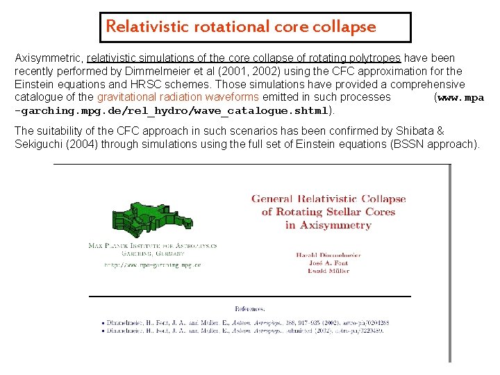
Relativistic rotational core collapse Axisymmetric, relativistic simulations of the core collapse of rotating polytropes have been recently performed by Dimmelmeier et al (2001, 2002) using the CFC approximation for the Einstein equations and HRSC schemes. Those simulations have provided a comprehensive catalogue of the gravitational radiation waveforms emitted in such processes (www. mpa -garching. mpg. de/rel_hydro/wave_catalogue. shtml). The suitability of the CFC approach in such scenarios has been confirmed by Shibata & Sekiguchi (2004) through simulations using the full set of Einstein equations (BSSN approach).

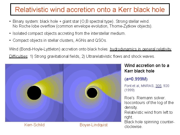
Relativistic wind accretion onto a Kerr black hole • Binary system: black hole + giant star (O, B spectral type). Strong stellar wind. No Roche lobe overflow (common envelope evolution, Thorne-Zytkow objects). • Isolated compact objects accreting from the interstellar medium. • Compact objects in stellar clusters, AGNs and QSOs. Wind (Bondi-Hoyle-Lyttleton) accretion onto black holes: hydrodynamics in general relativity. Difficulties: 1) Strong gravitational fields, 2) Ultrarelativistic flows and shock waves. Wind accretion on to a Kerr black hole (a=0. 999 M) Font et al, MNRAS, 305, 920 (1999) Kerr-Schild Boyer-Lindquist Roe’s Riemann solver. Isocontours of the log of the density. Relativistic wind from left to right. Black hole spinning counterclockwise.

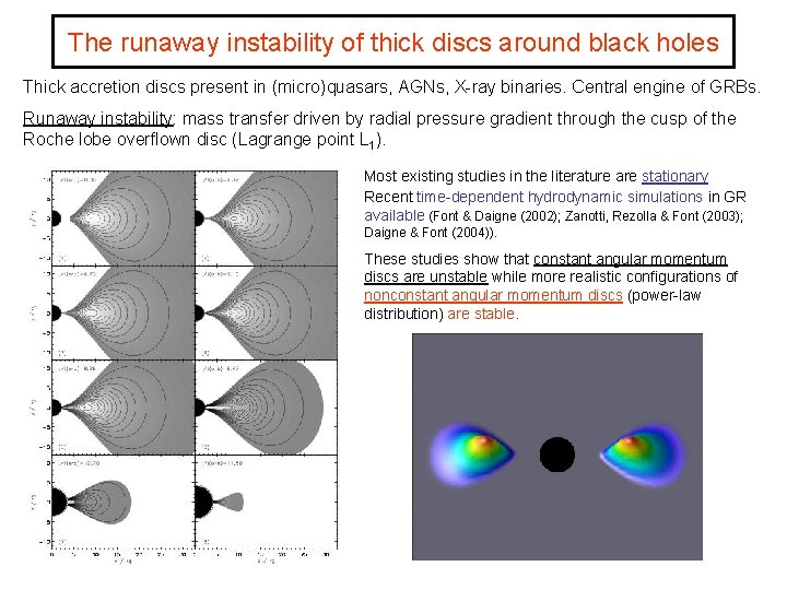
The runaway instability of thick discs around black holes Thick accretion discs present in (micro)quasars, AGNs, X-ray binaries. Central engine of GRBs. Runaway instability: mass transfer driven by radial pressure gradient through the cusp of the Roche lobe overflown disc (Lagrange point L 1). Most existing studies in the literature are stationary Recent time-dependent hydrodynamic simulations in GR available (Font & Daigne (2002); Zanotti, Rezolla & Font (2003); Daigne & Font (2004)). These studies show that constant angular momentum discs are unstable while more realistic configurations of nonconstant angular momentum discs (power-law distribution) are stable.

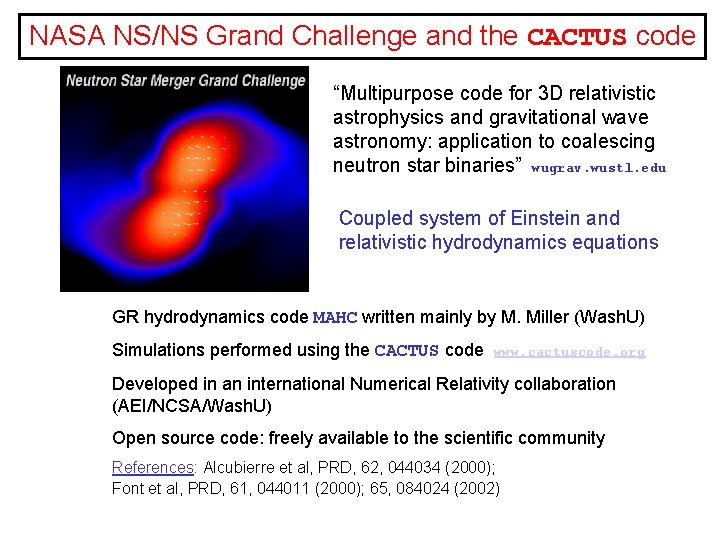
NASA NS/NS Grand Challenge and the CACTUS code “Multipurpose code for 3 D relativistic astrophysics and gravitational wave astronomy: application to coalescing neutron star binaries” wugrav. wustl. edu Coupled system of Einstein and relativistic hydrodynamics equations GR hydrodynamics code MAHC written mainly by M. Miller (Wash. U) Simulations performed using the CACTUS code www. cactuscode. org Developed in an international Numerical Relativity collaboration (AEI/NCSA/Wash. U) Open source code: freely available to the scientific community References: Alcubierre et al, PRD, 62, 044034 (2000); Font et al, PRD, 61, 044011 (2000); 65, 084024 (2002)

EU-TMR Network on Sources of Gravitational Radiation and the WHISKY code Whisky: a 3 D, parallel code in Cartesian coordinates, which solves the GR hydrodynamics equations using HRSC schemes www. eu-network. org (Main) institutions involved in the code development: AEI (Golm, Germany), SISSA (Trieste, Italy), University of Valencia (Spain), University of Thessaloniki (Greece) SPACETIME EVOLUTION Cartesian 3 D unigrid and with FMR (fixed mesh refinement). Implementation of AMR is in progress Iterative Crank-Nicholson scheme (2 nd order accurate in space and time), but also RK, Leapfrog, etc. HYDRODYNAMICS Different approximate Riemann solvers implemented: HLLE, Roe, Marquina. Slope limiters: MUSCL, MC and PPM. Optimal results are obtained with Marquina’s flux formula and the MC slope limiter (2 nd order away from local extrema) Polytropic and realistic Eo. S

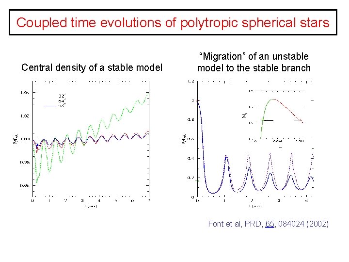
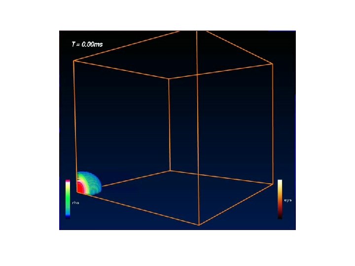
Coupled time evolutions of polytropic spherical stars Central density of a stable model “Migration” of an unstable model to the stable branch Font et al, PRD, 65, 084024 (2002)

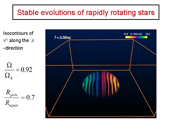
Stable evolutions of rapidly rotating stars Isocontours of vx along the x -direction

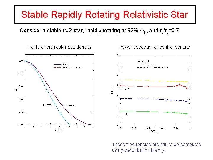
Stable Rapidly Rotating Relativistic Star Consider a stable G=2 star, rapidly rotating at 92% WK, and rp/re=0. 7 Profile of the rest-mass density Power spectrum of central density These frequencies are still to be computed using perturbation theory!

Conclusions • The hydrodynamic equations (either Newtonian or relativistic) constitute a Jjjj non-linear hyperbolic system, perhaps the archetypal example of hyperbolic model in astrophysics and cosmology. Aaa • There exist solid mathematical foundations and accurate numerical Aaa methodology imported from classical CFD and recently extended to Relativistic Astrophysics. • An emerging, “preferred” choice: high-resolution shock-capturing schemes based upon Riemann solvers, and written in conservation form. • Nowadays, computational general relativistic astrophysics is an increasingly important field of research in Numerical Relativity worldwide: gravitational stellar collapse, black hole formation, coalescence of compact binaries, gamma-ray bursts, … • In particular, hydrodynamical simulations in (static) curved backgrounds – test -fluid approximation – are routinely performed with satisfactory levels of accuracy.

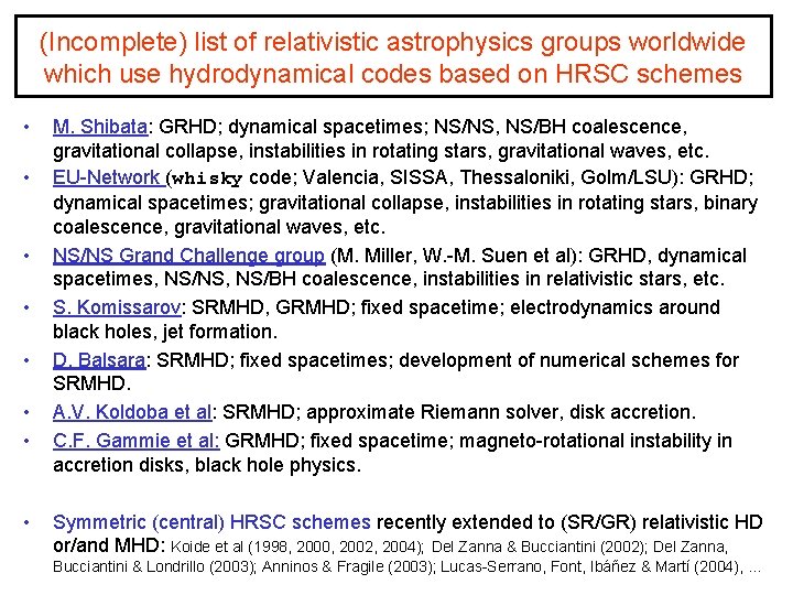
(Incomplete) list of relativistic astrophysics groups worldwide which use hydrodynamical codes based on HRSC schemes • • M. Shibata: GRHD; dynamical spacetimes; NS/NS, NS/BH coalescence, gravitational collapse, instabilities in rotating stars, gravitational waves, etc. EU-Network (whisky code; Valencia, SISSA, Thessaloniki, Golm/LSU): GRHD; dynamical spacetimes; gravitational collapse, instabilities in rotating stars, binary coalescence, gravitational waves, etc. NS/NS Grand Challenge group (M. Miller, W. -M. Suen et al): GRHD, dynamical spacetimes, NS/NS, NS/BH coalescence, instabilities in relativistic stars, etc. S. Komissarov: SRMHD, GRMHD; fixed spacetime; electrodynamics around black holes, jet formation. D. Balsara: SRMHD; fixed spacetimes; development of numerical schemes for SRMHD. A. V. Koldoba et al: SRMHD; approximate Riemann solver, disk accretion. C. F. Gammie et al: GRMHD; fixed spacetime; magneto-rotational instability in accretion disks, black hole physics. Symmetric (central) HRSC schemes recently extended to (SR/GR) relativistic HD or/and MHD: Koide et al (1998, 2000, 2002, 2004); Del Zanna & Bucciantini (2002); Del Zanna, Bucciantini & Londrillo (2003); Anninos & Fragile (2003); Lucas-Serrano, Font, Ibáñez & Martí (2004), …