Maximum Likelihood Haplotyping for General Pedigrees Fishelson M

"Maximum Likelihood Haplotyping for General Pedigrees. " Fishelson M. , Dovgolevsky N. and Geiger D. Human Heredity, 2005

Overview Genetic linkage: basic definitions Superlink: Preprocessing Finding optimal computation order Solving problem via Elim-Max Experimental results

Human Genome Most human cells contain 46 chromosomes: 2 sex chromosomes (X, Y): XY – in males. XX – in females. 22 pairs of chromosomes, named autosomes.

Genetic Information Gene – basic unit of genetic information. They determine the inherited characteristics. Genome – the collection of genetic information. Chromosomes – storage units of genes.

Genotype Vs. Phenotype Genotype - genetic constitution of an individual, inherited instructions it carries, which may or may not be expressed. Phenotype - any observed quality of an organism (such as morphology, development, or behavior)

Chromosome Logical Structure Genetic marker – a known DNA sequence, variation, which may arise due to mutation or alteration in the genomic loci, that can be observed. May be short (SNP) or long one (minisatellites) Locus – location of markers - fixed position on a chromosome Allele – one variant form of a marker. Locus 1 Possible Alleles: A 1, A 2 Locus 2 Possible Alleles: B 1, B 2, B 3

Alleles - the ABO (Blood types) locus example Multiple alleles: A, B, O. O is recessive to A. B is dominant over O. A and B are codominant.

Mendel’s first law Characters are controlled by pairs of genes which separate during the formation of the reproductive cells (meiosis) Aa A a

Sexual Reproduction Meiosis

Mendel’s second law When two or more pairs of genes segregate simultaneously, they do so independently. A a; B b AB PAB= PA PB Ab PAb=PA Pb a. B ab Pa. B=Pa PB Pab=Pa Pb

Hardy–Weinberg equilibrium genotype frequencies in a population remain constant or are in equilibrium from generation to generation unless specific disturbing influences are introduced f(B) = p f(b)=q final three possible genotypic frequencies in the offspring: f(BB)=p^2 f(Bb)=2 pq f(bb)=q^2

Recombination During Meiosis Genetic recombination is the process by which a strand of genetic material (usually DNA; but can also be RNA) is broken and then joined to a different DNA molecule. In humans recombination commonly occurs during meiosis as chromosomal crossover between paired chromosomes. Recombinant gametes

Linkage 2 genes on separate chromosomes assort independently at meiosis Recombination can occur with small probability at any location along chromosome 2 genes far apart on the same chromosome can also assort independently at meiosis. 2 genes close together on the same chromosome pair do not assort independently at meiosis. A recombination frequency << 50% between 2 genes shows that they are linked – they are inherited together.

Linkage Maps Let U and V be 2 genes on the same chromosome. In every meiosis, chromatids cross over at random along the chromosome. If the chromatids cross over between U & V, then a recombinant is produced.

Relative distance between two genes - can be calculated using the offspring of an organism showing two linked genetic traits, and finding the percentage of the offspring where the two traits do not run together. The higher the percentage of descendants that does not show both traits, the further apart on the chromosome they are.

Recombination Fraction • The recombination fraction between two loci is the percentage of times a recombination occurs between the two loci. • is a monotone, nonlinear function of the physical distance separating the loci on the chromosome.

Centimorgan (c. M) 1 c. M (or 1 genetic map unit, m. u. ) is the distance between genes for which the recombination frequency is 1%, that is genes for which one product of meiosis in 100 is recombinant.

Haplotype - a combination of alleles at multiple linked loci that are transmitted together. Haplotype may refer to as few as two loci or to an entire chromosome depending on the number of recombination events that have occurred between a given set of loci.

Haplotype Resolution Given the genotypes for a number of individuals, the haplotypes can be inferred by haplotype resolution or haplotype phasing techniques. These methods work by applying the observation that certain haplotypes are common in certain genomic regions. Methods: - compinatorial approach - likelihood functions An organism's genotype may not uniquely define its haplotype

SUPERLINK: Multipoint linkage analisys – estimate recombination fraction between a disease gene and known loci on the chromosome. Haplotyping problem - infer the two haplotypes of each individual from the measured unordered genotypes (using pedigree genotype data and population genotype data) Both problems can be defined via maximizing a suitable likelihood function.

Bayesian networks for representation of pedigree data Allow to represent pedigrees in detailed manner Allow to encode independence assumptions Pedigree – defines a joint distribution over the genotypes and phenotypes of the individuals represented in the pedigree.

Random variables representing a pedigree Separate single-locus allele lists for the two haplotypes (paternal and maternal) Genetic Loci: Gi, jp, Gi, jm – specific alleles of locus j in individual i's paternal and maternal haplotypes Phenotypes: Pi, j – for each individual i and phenotype j denotes the value of phenotype for individual i. Selector variable: Si, jp, Si, jm – denote the selection made by meiosis that resulted in i's genetic makeup a locus j. Formally, if a denotes i's father, then Gi, jp = Ga, jp if Si, jp = 0 Gi, jp = Ga, jm if Si, jp = 1

Local probability tables: Transmission models: Pr(Gi, jp|Ga, jp, Ga, jm, Si, jp), Pr(Gi, jm|Gb, jp, Gb, jm, Si, ) where a and b are i's parents in pedigree. These tables are jm deterministic, namely, consist solely of 0 and 1. The first probability table equals 1, if Gi, jp=Ga, jp and Si, jp=0, or if Gi, jp=Ga, jm and Si, jp=1. In all other cases, this probability table equals 0. The second probability table is defined analogously. Penetrance model (Penetrance - the proportion of individuals carrying a particular variation of a gene (an allele or genotype) that also express a particular trait (the phenotype)) or Marker model: Pr(Pi, j| Gi, jp, Gi, jm) These tables are also deterministic. The probability table equals 1 if Pi, j= (Gi, jp, Gi, jm), or if Pi, j=(Gi, jm, Gi, jp). Otherwise it equals 0. The assumption underlying these models is that there are no measurement errors.

Local probability tables: Recombination model: Pr(Si, 1 p) = Pr(Si, 1 m) = 0. 5, Pr(Si, jp|Si, j-1 p, j-1) and Pr(Si, jm|Si, j-1 m, j-1), where j-1 is the known or unknown recombination fraction between locus j-1 and locus j. The recombination fractions between the markers are specified by the user in the input to SUPERLINK. These recombination models do not take genetic interference into account. General population allele frequencies: Pr(Gi, jp), Pr(Gi, jm), when i is a founder (whose biological parents are not included in the pedigree). The use of these models is based on the assumptions of Hardy. Weinberg and linkage equilibriums. Each of these probability tables is called a factor.

A fragment of a Bayesian network representation of parents-child interaction in a 3 -loci analysis.

Superlink solves: For haplotyping – Most Probable Explanation problem: Superlink represents joint distribution over selector variables (S) and the genetic loci variables of founders (F), and nonfounders (N) in factored form:

Haplotyping problem A maximum-likelihood haplotype configuration of a pedigree is a maximum-likelihood assignment to all the genetic loci variables: Since we are interested in determining the most likely gene flow as well, we seek a joint maximum-likelihood assignment to the selector variables and the genetic loci variables of founders Since genetic loci variables of non-founders, N, are a function of the genetic loci variables of founders and the selector variables, solving equation above is equivalent to:

Algorithm: Preprocessing Value elimination Variable trimming Allele recording Finding optimal computation order Solving problem via Elim-Max (elim-mpe) combined with conditioning

Value elimination 1 st step – performed directly on the graph representation of pedigree, before transforming it into Bayesian network. 2 nd step – performed on the local probability tables that annotate nodes of the constructed Bayesian network.

st 1 step - based on the fact, that possible genotypes of an individual can be inferred from the genotypes of one's relatives. Downward update: the child is updated according to parent Ex. - a child can only have allele 1 or 2 in paternal haplotype of this locus

st 1 step Upward update: parent is updated according to the children Ex. - both children got allele 1 from their mother. So, father's genotype must be 3|4 These updates work in local manner, but when each update is propagated through the pedigree graph, it results in global update.

nd 2 Step Value of certain variable is invalid, if all entries of some probability table that corresponds to that value of that variable equal zero. Variable trimming Variables that correspond to leaves in the Bayesian network for which no data exists can be trimmed without altering likelihood computation.

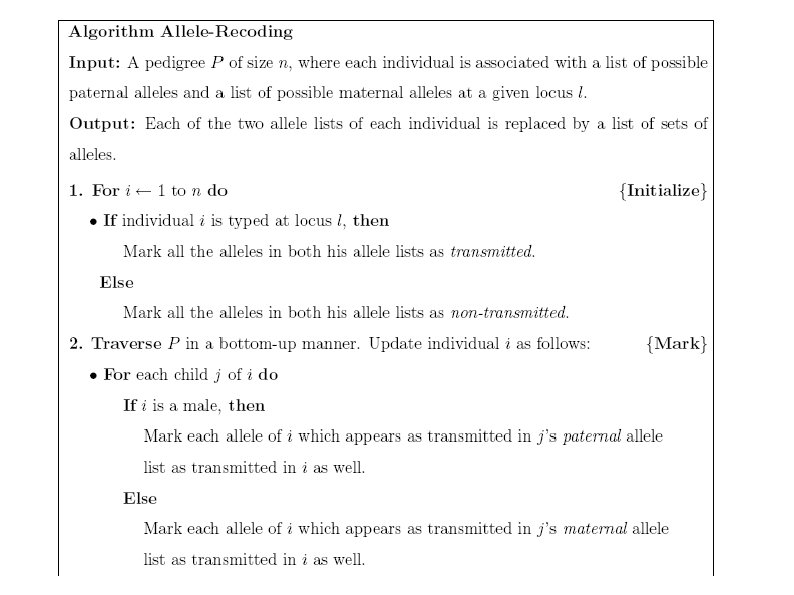
Allele recording Reduces the number of genotypes that need to be summed over, and hence, accelerates of computations. One method is lumping alleles that do not appear in the pedigree into a single allele whose population frequency is the sum of frequencies of the lumped alleles (Lange et al. , 1988; Schaffer, 1996). A more efficient method, which recodes the paternal and maternal allele lists of each individual separately, has been suggested by O'connell and Weeks (1995), and implemented in vitesse. The allele recoding algorithm implemented in superlink is based on the ideas of set-recoding and fuzzy inheritance defined in vitesse.

allele-recoding algorithm An allele is defined to be transmitted if the following two conditions are fulfilled: (I) the allele appears in the ordered genotype list of a typed descendant D of P, as inherited from P; (ii) there is some path from P to D containing only untyped descendants in the pedigree, namely, D is the nearest typed descendant of P on that path. The remaining alleles are defined to be non-transmitted. In terms of determining recombination events, a person's nontransmitted alleles are indistinguishable from one another by data, and can therefore be combined into a single representative allele.

Algorithm allele-recording p 2

The probability of the assignment found for the regular case (without allele recoding) is the same as the one found in the case of allele recoding.

Computation order Main approaches: Elston-Steward algorithm – processes one nuclear family after another. Good for large pedigrees with a few markers. Lander-Green algorithm – processes one locus after another. Good for small to medium-sized pedigrees with large number of markers. Superlink uses novel approach. In Superlink problem is reduced to operations on a moralized graph of Bayesian network.

When a vertex is eliminated from the graph, its set of neighbors are connected to form a clique. The cost of eliminating vertex v from graph Gi is where NGi(v) represents the set of neighbors of v including v itself, and w(v) is the weight of v, namely, the number of possible values of variable Xv. In the case when there is no memory limitation, we aim to find an elimination order ^Xa which satisfies ^Xa = arg mina C(Xa), where and a denotes a permutation on {1, . . . , n}. Gi, i = 2, . . . , n denotes the sequence of residual graphs obtained from a given graph G 1 = G by eliminating its vertices in the order Xa(1), . . Xa(i-1).

Cost Function C(Xa) – cost function (total state space) – approximated measure of the time and space complexity of the computation. If heaviest clique created doesn't fit into memory – conditioning is needed.

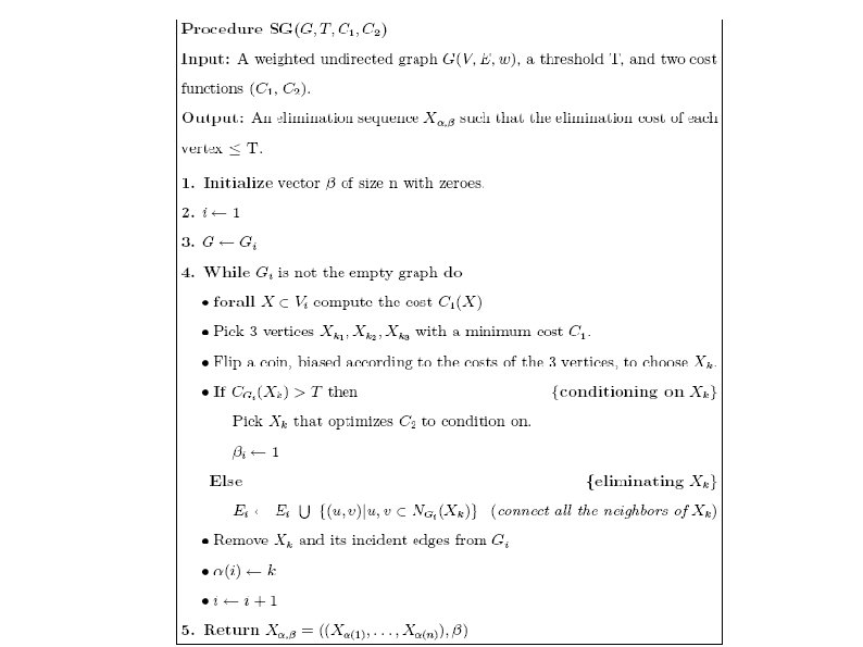
Cost function for conditioning Let β = (β 1, …βn) be a vector where βi €{0, 1}. A constrained elimination sequence Xα, β = ((Xα(1), …, Xα(n), β) is a sequence of vertices along the binary vector β such that vertex Xα(i) is eliminated if βi = 0 and conditioned on if βi=1. Goal – to find (for memory threshold T)

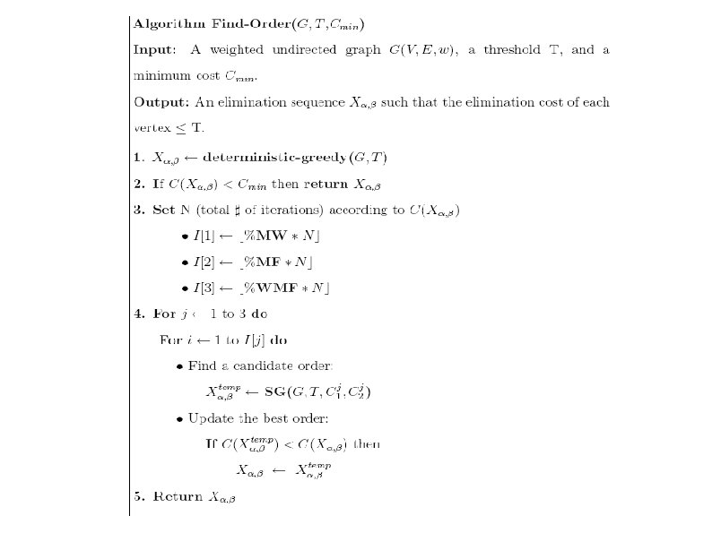
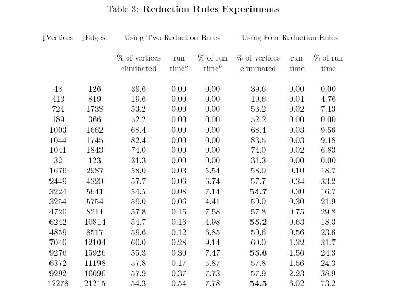
Algorithm for finding a combined order of elimination and conditioning (for both haplotyping and likelihood computation) Preprocessing step – application of reduction rules (initially designed for weighted treewidth problem. They can significantly reduce size of the graph) Application of several stochastic-greedy algorithms

Reduction rules Variable low – represents the largest lower bound known for the weighted treewidth of the original graph. Simplicial rule: Let v be a simplicial vertex in Gi, namely its set of neighbors form a clique. The simplicial rule removes v from the graph, and updates the variable low: low = max(low; nw(v)). Almost simplicial rule: A vertex v is called an almost simplicial vertex in Gi if all its neighbors, except one u, form a clique. Vertex v is removed if low>= nw(v) and w(v) >=w(u). nw(v) denotes product

Stochastic-greedy algorithms All based on the same procedure SG() (see next slide) Input: weighted undirected graph G(V, E, w) Threshold T (memory limitation) cost functions C 1 and C 2 (vary between three algorithms) Acording to C 1 next vertex to be eliminated is chosen. Acording to C 2 next vertex to be conditioned on is chosen. Procedure runs many times, each times finds new elimination order and compares it to previous one

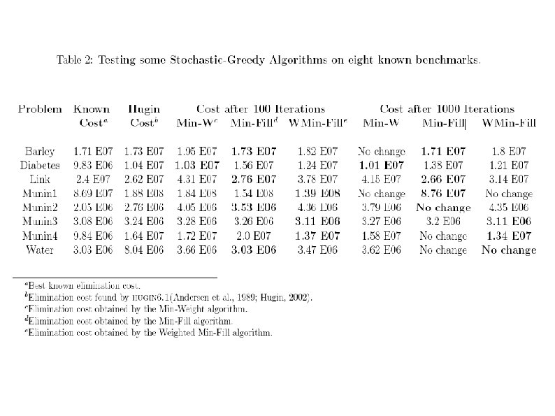
Three algorithms Min-Weight (Win-W): C 1 – product of weights of vertex's neighbours Min-Fill: C 1 – number of edges that need to be added to the graph after elimination of the vertex - set of neighbours of X in Gi , - # of neighbours Weighted Min-Fill (Wmin-Fill): Weight of an edge – product of weights of its constituent vertices. C 1 - sum of weights of the edges that need to be added due to vertex's elimination - functions in Gi that include X

Three algorithms Neither of the algorithms is better than others in all cases, so each of them is run a certain percentage of total optimization time: %MW, %MF, %WMF – percentage of iterations spent on running Min-Weight, Min-Fill and Weighted Min-Fill. N – total number of iterations – estimated according to the complexity of the problem at hand, which is estimated by cost of elimination found by deterministic-greedy Min. Weight algorithm.

Deterministic-greedy Min-Weight Deterministic each iteration chooses to eliminate vertex with a minimal elimination cost according to the Min. Weight cost function Stochastic each interation flips a coin to determine which vertex out of three chosen to eliminate.

Experimental results Evaluation of the optimization algorithm Stochastic algorithm Benchmarks Total running time Reduction rules Evaluation of the haplotyping algorithm

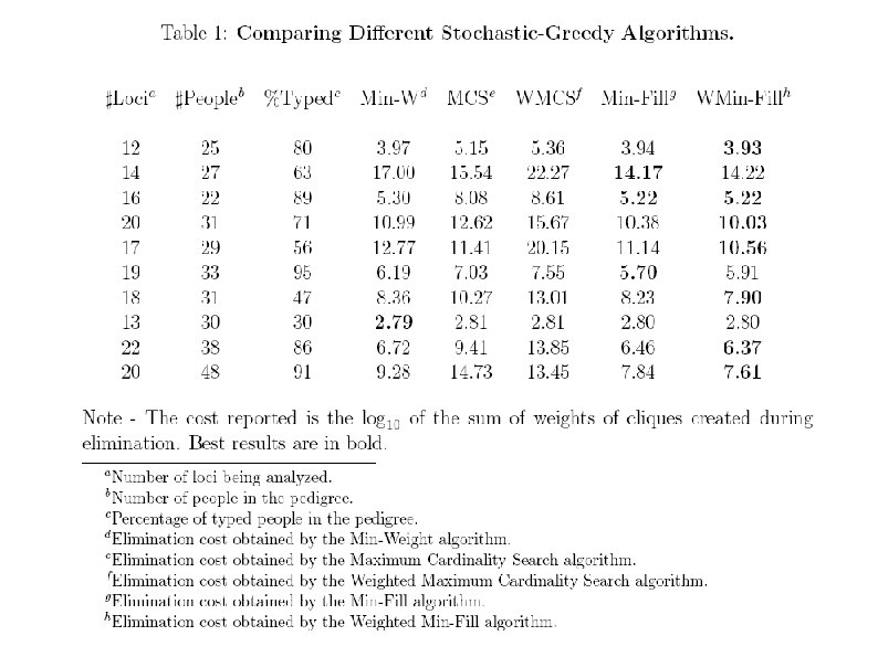
Distribution of algorithms that found the lower cost Min-Weight heuristic does not provide as good results as Weighted Min-Fill and Min-Fill, but it is the fastest and works well when conditioning is needed. The MCS and Weighted-MCS heuristics have been found to hardly contribute when applied after the Min-Weight and thus are not implemented

Comparison of likelihood computation using old and new(1. 4) version of Superlink

Simulation study Superlink haplotyping algorithm was tested on a complex pedigree of moderate size (Lin, 1996). So far, only an approximate haplotype analysis was possible for this pedigree. Superlink obtained a maximum likelihood haplotype configuration in several minutes. This pedigree consists of 27 individuals and is highly inbred. Genehunter removes 12 individuals from the pedigree in order to perform the computations. At the time, no previous exact algorithm could produce the maximum likelihood haplotype conguration for this pedigree.

Simulation study

Testing correctness Implementing three independent versions of the algorithm, and comparing the results obtained by all three versions. Each version was implemented by different people, to assure an independent evaluation. Correctness: the software finds a haplotype configuration of maximum likelihood given the assumptions of Hardy-Weinberg and Linkage equilibrium. Tested 60 data sets consisting of 5 to 150 individuals and up to 200 markers. In all tested data sets, all three versions produced haplotype configurations with the same likelihood. There is usually more than one maximum-likelihood haplotype configuration, and hence, various algorithms often produce different haplotype configurations.

Testing accuracy Using Superlink, approximated haplotyping can be compared with the optimal solution on larger pedigrees than was previously possible. This experiment tested the accuracy of a state of the art program that uses MCMC, called simwalk 2. 75 random data sets consisting of 15 to 50 individuals and up to 10 markers were tested. Simwalk 2 found a maximal likelihood assignment in 45 out of the 75 data sets. In the other 30 data sets, the average diference in the loglikelihood of the assignment found by simwalk 2 compared to the maximal likelihood assignment was merely 1%

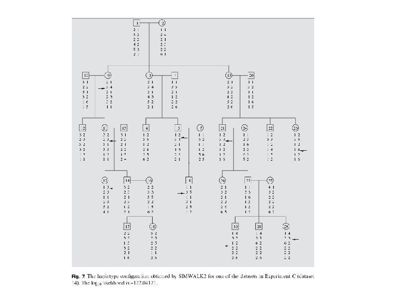
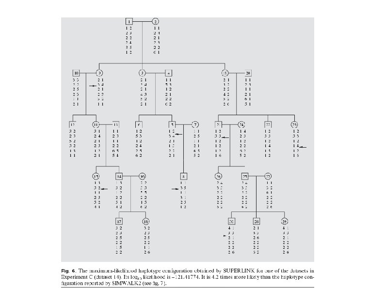
Testing accuracy Example of different outputs by SIMWALK 2 and SUPERLINK. The two haplotype configurations are quite similar. Many of the differences involve different phases in the haplotypes of founders. Such information can not be discerned by the data, and hence, such differences are meaningless. However, the haplotype configuration found by SIMWALK 2 contains 9 recombination events whereas the haplotype configuration found by SUPERLINK contains merely 7 recombination events. The positions of 5 of the recombination events found by both programs are the same. The other 2 recombination events found by SUPERLINK are in different positions than those found by SIMWALK 2. The likelihood of the haplotype configuration found by SUPERLINK is 4. 2 times higher than the one reported by SIMWALK 2.

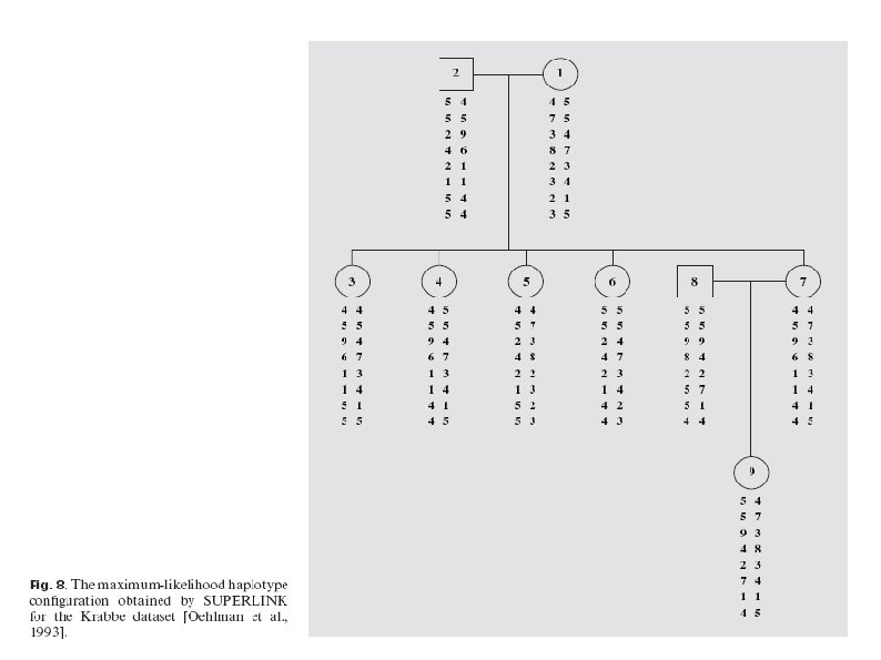
Published Disease Data Two published data sets from a study of the Krabbe disease , and from a study on Episodic Ataxia (EA) were analysed. The first data set consists of 9 individuals typed at 8 polymorphic markers. The second data set consists of 29 individuals, which are all typed at 9 polymorphic markers except for the first two generation founders. For the Krabbe data set, the most likely haplotype conguration obtained by Superlink is identical to the one obtained by MCMC via simwalk 2, by Lin and Speed, and by pedphase. For the Episodic Ataxia data set, the most probable conguration difers from the one obtained by simwalk 2 in the position of one recombination event. The only dierence is the genotype phase in the fourth marker of individuals 1007 and 113. This conguration is also very similar to the one found by Lin and Speed.