Maximum Likelihood Phylogeny Estimation Neelima Lingareddy Maximum Likelihood

Maximum Likelihood: Phylogeny Estimation Neelima Lingareddy

Maximum Likelihood • This method was first proposed by the English statistician R. A. Fisher in 1922. • His advisors didn’t think it was such a useful idea!

What is maximum likelihood? • The likelihood is the probability of the data given the model • The probability of observing the data under the assumed model will change depending on the parameter values of the model. • The aim of maximum likelihood is to choose the value of the parameter that maximizes the probability of finding the data.

Three main components of maximum likelihood • Data • A model describing the probability of observing the data • A criterion that allows us to move from the data and model to an estimate of the parameters of the model.

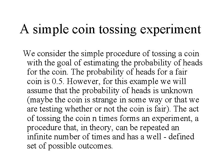
A simple coin tossing experiment We consider the simple procedure of tossing a coin with the goal of estimating the probability of heads for the coin. The probability of heads for a fair coin is 0. 5. However, for this example we will assume that the probability of heads is unknown (maybe the coin is strange in some way or that we are testing whether or not the coin is fair). The act of tossing the coin n times forms an experiment, a procedure that, in theory, can be repeated an infinite number of times and has a well - defined set of possible outcomes.

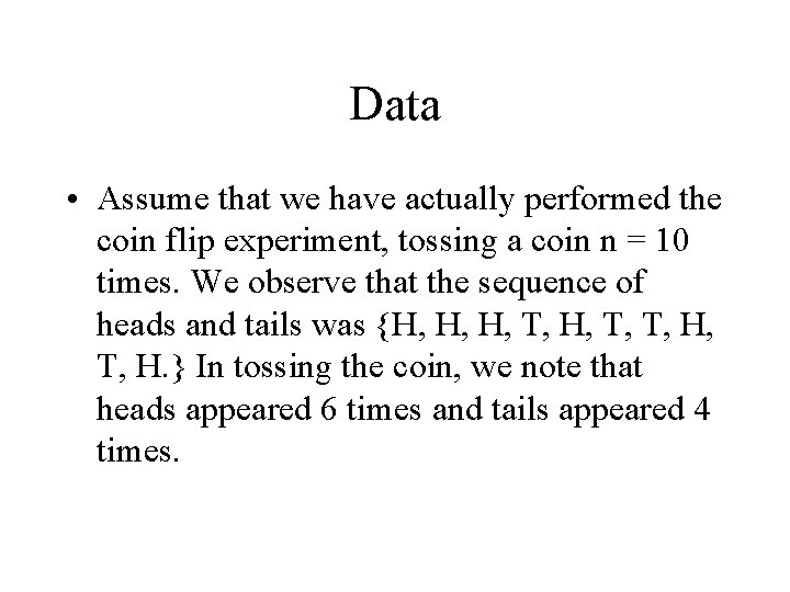
Data • Assume that we have actually performed the coin flip experiment, tossing a coin n = 10 times. We observe that the sequence of heads and tails was {H, H, H, T, T, H, T, H. } In tossing the coin, we note that heads appeared 6 times and tails appeared 4 times.

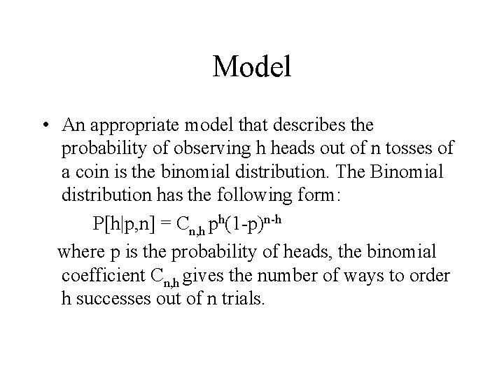
Model • An appropriate model that describes the probability of observing h heads out of n tosses of a coin is the binomial distribution. The Binomial distribution has the following form: P[h|p, n] = Cn, h ph(1 -p)n-h where p is the probability of heads, the binomial coefficient Cn, h gives the number of ways to order h successes out of n trials.

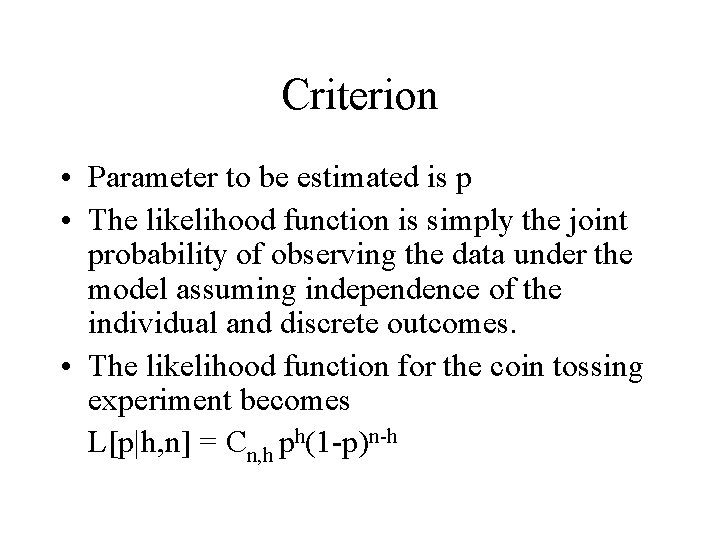
Criterion • Parameter to be estimated is p • The likelihood function is simply the joint probability of observing the data under the model assuming independence of the individual and discrete outcomes. • The likelihood function for the coin tossing experiment becomes L[p|h, n] = Cn, h ph(1 -p)n-h

Maximum Likelihood: Calculations • The log-likelihood can be written as log. L[p|h, n] = log(n!) – log(h!) – log((n-h)!) + hlog p +(n-h)log(1 -p) • It makes calculations easier • The factorials do not change for different values of p. So they can be ignored (and usually are!)

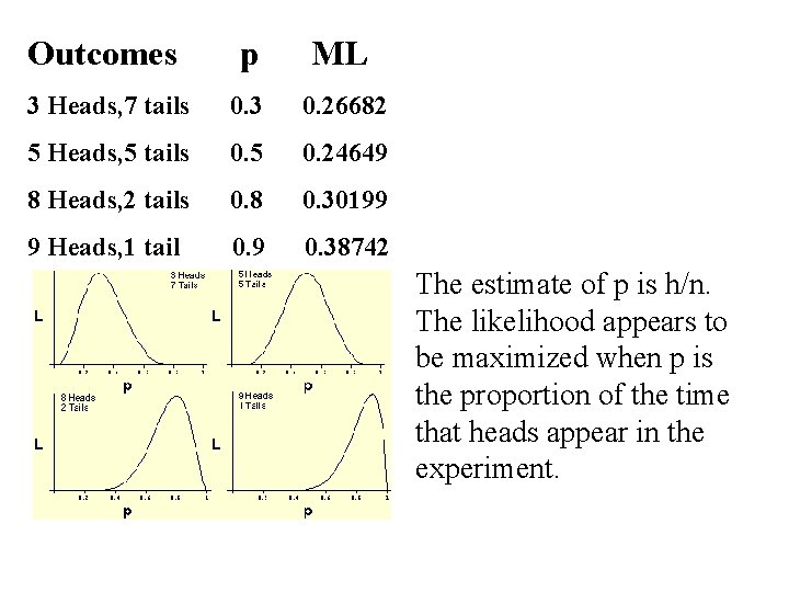
Outcomes p ML 3 Heads, 7 tails 0. 3 0. 26682 5 Heads, 5 tails 0. 5 0. 24649 8 Heads, 2 tails 0. 8 0. 30199 9 Heads, 1 tail 0. 9 0. 38742 The estimate of p is h/n. The likelihood appears to be maximized when p is the proportion of the time that heads appear in the experiment.

Phylogenetics • Study of different life forms (process of evolution) • Recent field and received a huge push forward due to stronger and faster computers • Reconstruct the evolutionary relationship between species and to estimate the time of divergence between two organisms since they shared a last common ancestor. • Phylogenetic analysis of DNA or protein sequences has become an important tool for studying the evolutionary history of organisms from bacteria to humans.

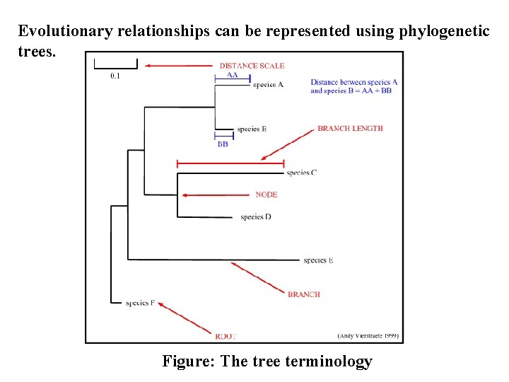
Evolutionary relationships can be represented using phylogenetic trees. Figure: The tree terminology

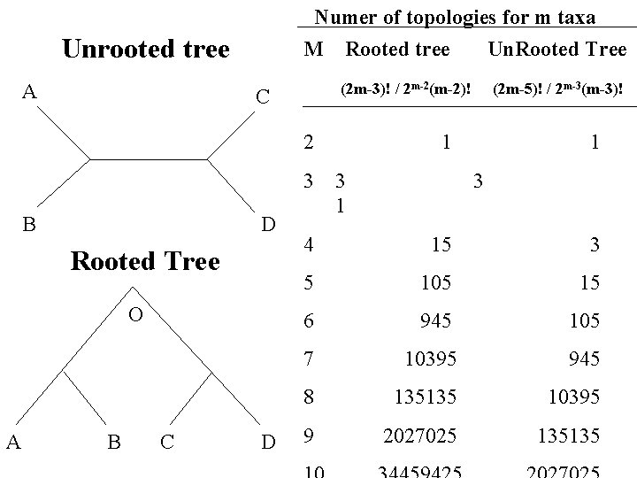
Numer of topologies for m taxa Unrooted tree A M Rooted tree Un. Rooted Tree C (2 m-3)! / 2 m-2(m-2)! (2 m-5)! / 2 m-3(m-3)! 2 1 B D Rooted Tree 3 3 1 4 15 3 5 105 15 O 6 945 105 7 10395 945 8 135135 10395 A B C D 9 2027025 135135

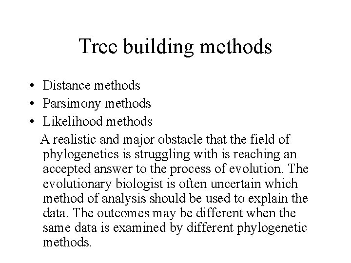
Tree building methods • Distance methods • Parsimony methods • Likelihood methods A realistic and major obstacle that the field of phylogenetics is struggling with is reaching an accepted answer to the process of evolution. The evolutionary biologist is often uncertain which method of analysis should be used to explain the data. The outcomes may be different when the same data is examined by different phylogenetic methods.

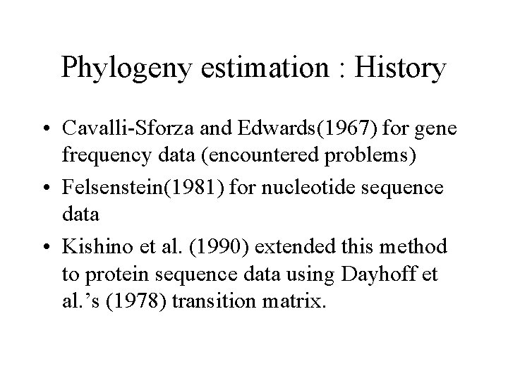
Phylogeny estimation : History • Cavalli-Sforza and Edwards(1967) for gene frequency data (encountered problems) • Felsenstein(1981) for nucleotide sequence data • Kishino et al. (1990) extended this method to protein sequence data using Dayhoff et al. ’s (1978) transition matrix.

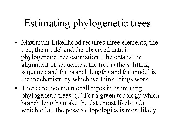
Estimating phylogenetic trees • Maximum Likelihood requires three elements, the tree, the model and the observed data in phylogenetic tree estimation. The data is the alignment of sequences, the tree is the splitting sequence and the branch lengths and the model is the mechanism by which we think things work. • There are two main challenges in estimating phylogenetic trees: (1) For a given topology which branch lengths make the data most likely, (2) which of all the possible topologies is most likely.

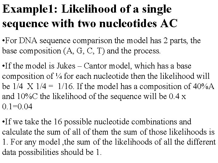
Example 1: Likelihood of a single sequence with two nucleotides AC • For DNA sequence comparison the model has 2 parts, the base composition (A, G, C, T) and the process. • If the model is Jukes – Cantor model, which has a base composition of ¼ for each nucleotide then the likelihood will be 1/4 X 1/4 = 1/16. If the model has a composition of 40%A and 10%C the likelihood of the sequence will be 0. 4 x 0. 1=0. 04 • If we take the 16 possible nucleotide combinations and calculate the sum of all of them the sum of those likelihoods is 1. For any model , the sum of the likelihoods of all the different data possibilities should be 1.

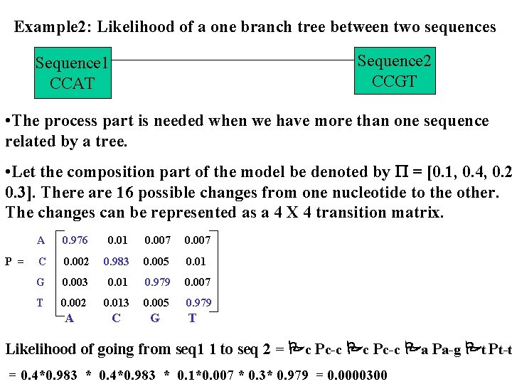
Example 2: Likelihood of a one branch tree between two sequences Sequence 2 Sequence 1 CCAT CCGT • The process part is needed when we have more than one sequence related by a tree. • Let the composition part of the model be denoted by = [0. 1, 0. 4, 0. 2 0. 3]. There are 16 possible changes from one nucleotide to the other. The changes can be represented as a 4 X 4 transition matrix. A 0. 976 0. 01 0. 007 P = C 0. 002 0. 983 0. 005 0. 01 G 0. 003 0. 01 0. 979 0. 007 T 0. 002 0. 013 0. 005 0. 979 A C G T Likelihood of going from seq 1 1 to seq 2 = c Pc-c a Pa-g t Pt-t = 0. 4*0. 983 * 0. 1*0. 007 * 0. 3* 0. 979 = 0. 0000300

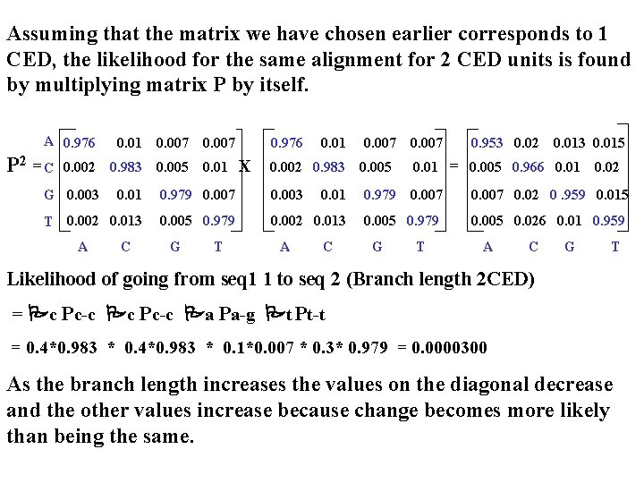
Assuming that the matrix we have chosen earlier corresponds to 1 CED, the likelihood for the same alignment for 2 CED units is found by multiplying matrix P by itself. A 0. 976 0. 01 0. 007 0. 976 0. 01 0. 007 0. 953 0. 02 0. 013 0. 015 P 2 = C 0. 002 0. 983 0. 005 0. 01 X 0. 002 0. 983 0. 005 0. 01 = 0. 005 0. 966 0. 01 0. 02 G 0. 003 0. 01 0. 979 0. 007 0. 02 0. 959 0. 015 0. 002 0. 013 0. 005 0. 979 T 0. 002 0. 013 0. 005 0. 979 0. 005 0. 026 0. 01 0. 959 A C G T Likelihood of going from seq 1 1 to seq 2 (Branch length 2 CED) = c Pc-c a Pa-g t Pt-t = 0. 4*0. 983 * 0. 1*0. 007 * 0. 3* 0. 979 = 0. 0000300 As the branch length increases the values on the diagonal decrease and the other values increase because change becomes more likely than being the same.

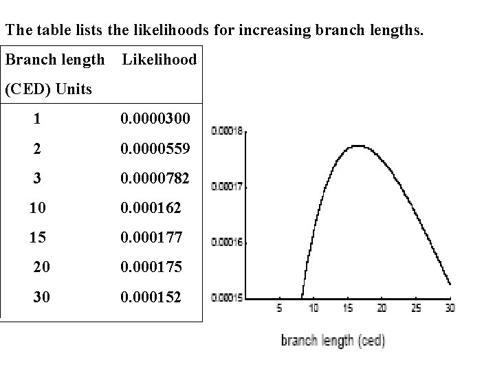
The table lists the likelihoods for increasing branch lengths. Branch length Likelihood (CED) Units 1 0. 0000300 2 0. 0000559 3 0. 0000782 10 0. 000162 15 0. 000177 20 0. 000175 30 0. 000152

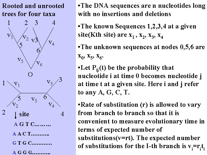
Rooted and unrooted trees for four taxa 1 2 3 4 v 1 v 2 v 3 5 6 v 4 v 5 1 5 2 v 3 3 v 1 v 2 v 5 6 v 4 site A G T C……… A A C T………. . G T G C………… A G G G………. . • The known Sequences 1, 2, 3, 4 at a given site(Kth site) are x 1 , x 2, x 3, x 4 • The unknown sequences at nodes 0, 5, 6 are x 0, x 5, x 6. v 6 O • The DNA sequences are n nucleotides long with no insertions and deletions 4 • Let Pij(t) be the probability that nucleotide i at time 0 becomes nucleotide j at time t at a given site. Here i and j refer to any A, G, C, T. • Rate of substitution (r) is allowed to vary from branch to branch so that it is convenient to measure evolutionary time in terms of expected number of substitutions(v=rt). The expected number of substitutions for the I-th branch is vi=riti

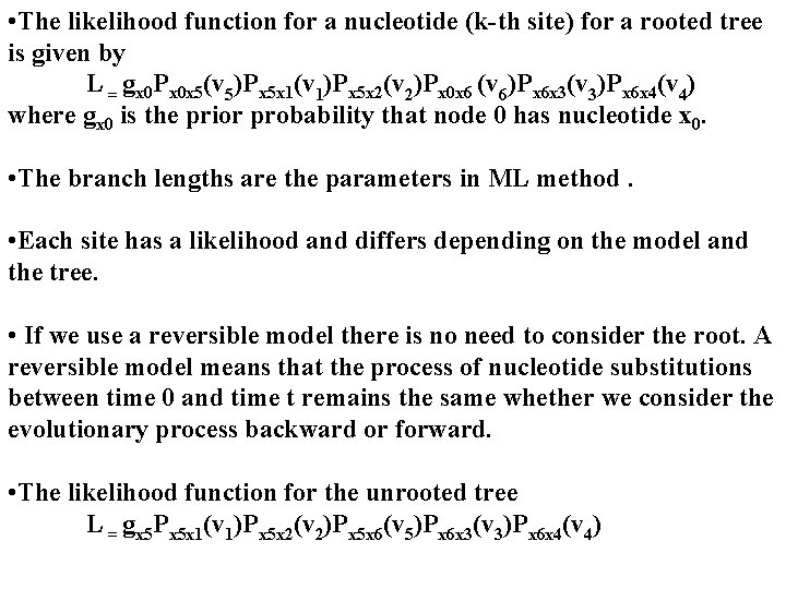
• The likelihood function for a nucleotide (k-th site) for a rooted tree is given by L = gx 0 Px 0 x 5(v 5)Px 5 x 1(v 1)Px 5 x 2(v 2)Px 0 x 6 (v 6)Px 6 x 3(v 3)Px 6 x 4(v 4) where gx 0 is the prior probability that node 0 has nucleotide x 0. • The branch lengths are the parameters in ML method. • Each site has a likelihood and differs depending on the model and the tree. • If we use a reversible model there is no need to consider the root. A reversible model means that the process of nucleotide substitutions between time 0 and time t remains the same whether we consider the evolutionary process backward or forward. • The likelihood function for the unrooted tree L = gx 5 Px 5 x 1(v 1)Px 5 x 2(v 2)Px 5 x 6(v 5)Px 6 x 3(v 3)Px 6 x 4(v 4)

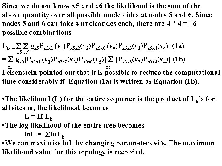
Since we do not know x 5 and x 6 the likelihood is the sum of the above quantity over all possible nucleotides at nodes 5 and 6. Since nodes 5 and 6 can take 4 nucleotides each, there are 4 * 4 = 16 possible combinations Lk = gx 5 Px 5 x 1 (v 1)Px 5 x 2(v 2)Px 5 x 6 (v 5)Px 6 x 3(v 3)Px 6 x 4(v 4) (1 a) x 5 x 6 = gx 5[Px 5 x 1 (v 1)Px 5 x 2(v 2)Px 5 x 6(v 5)] [Px 6 x 3(v 3)Px 6 x 4(v 4)] (1 b) x 5 x 6 Felsenstein pointed out that it is possible to reduce the computational time considerably if Equation (1 a) is written as Equation (1 b). • The likelihood (L) for the entire sequence is the product of Lk’s for all sites m, the likelihood becomes L = Lk • The log likelihood of the entire tree becomes ln. L = ln. Lk • We can maximize ln. L by changing parameters vi’s. The maximum likelihood value for this topology is recorded.

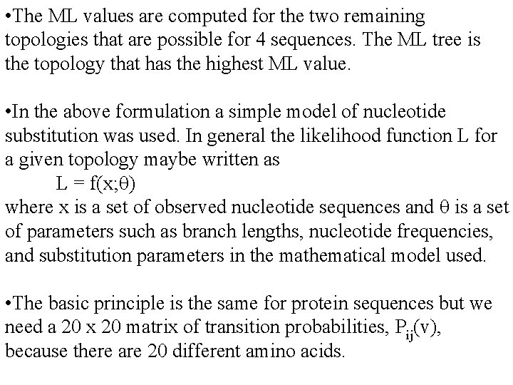
• The ML values are computed for the two remaining topologies that are possible for 4 sequences. The ML tree is the topology that has the highest ML value. • In the above formulation a simple model of nucleotide substitution was used. In general the likelihood function L for a given topology maybe written as L = f(x; ) where x is a set of observed nucleotide sequences and is a set of parameters such as branch lengths, nucleotide frequencies, and substitution parameters in the mathematical model used. • The basic principle is the same for protein sequences but we need a 20 x 20 matrix of transition probabilities, Pij(v), because there are 20 different amino acids.

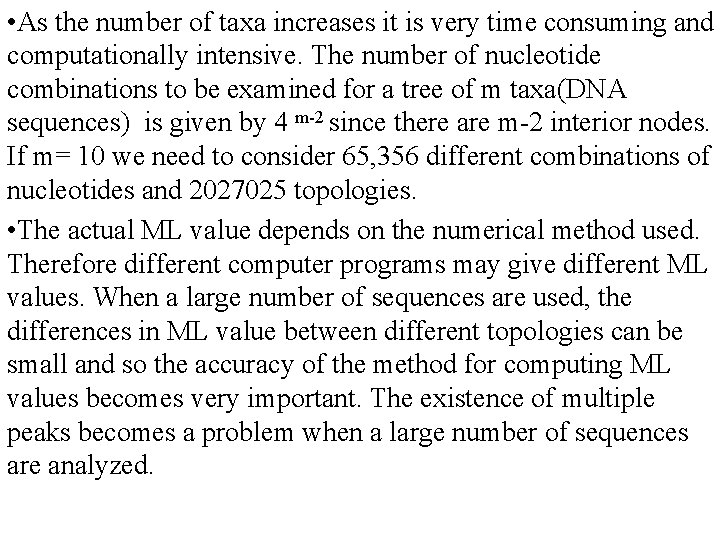
• As the number of taxa increases it is very time consuming and computationally intensive. The number of nucleotide combinations to be examined for a tree of m taxa(DNA sequences) is given by 4 m-2 since there are m-2 interior nodes. If m= 10 we need to consider 65, 356 different combinations of nucleotides and 2027025 topologies. • The actual ML value depends on the numerical method used. Therefore different computer programs may give different ML values. When a large number of sequences are used, the differences in ML value between different topologies can be small and so the accuracy of the method for computing ML values becomes very important. The existence of multiple peaks becomes a problem when a large number of sequences are analyzed.

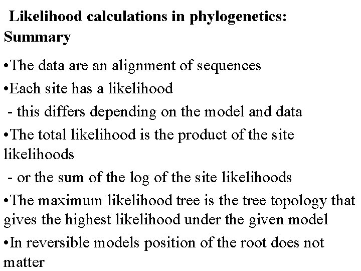
Likelihood calculations in phylogenetics: Summary • The data are an alignment of sequences • Each site has a likelihood - this differs depending on the model and data • The total likelihood is the product of the site likelihoods - or the sum of the log of the site likelihoods • The maximum likelihood tree is the tree topology that gives the highest likelihood under the given model • In reversible models position of the root does not matter