Leastsquares Maximum likelihood and Bayesian methods Xuhua Xia

Least-squares, Maximum likelihood and Bayesian methods Xuhua Xia xxia@uottawa. ca http: //dambe. bio. uottawa. ca

Bayesian inference: Basic terms • Conditional probability, e. g. , p(P|C) = 10/100 • Joint probability • Marginal probability • Prior: Prior probability distribution • Posterior: Posterior probability distribution Cancer(C) Healthy(H) Sum Positive(P) Negative(N) Sum Slide 2

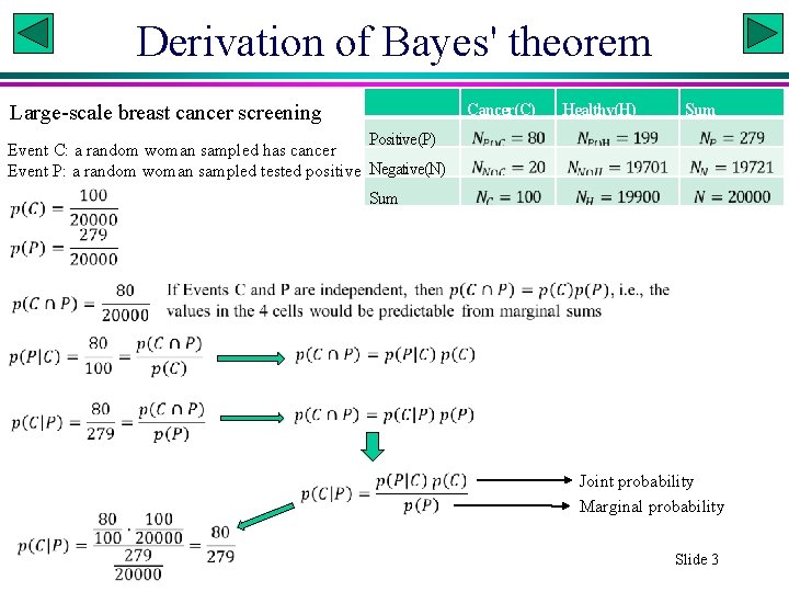
Derivation of Bayes' theorem Large-scale breast cancer screening Cancer(C) Healthy(H) Sum Positive(P) Event C: a random woman sampled has cancer Event P: a random woman sampled tested positive Negative(N) Sum Joint probability Marginal probability Slide 3

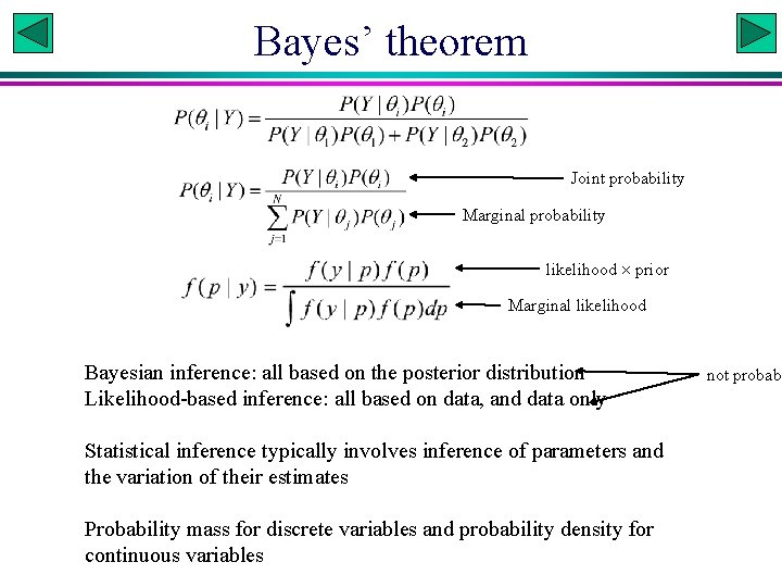
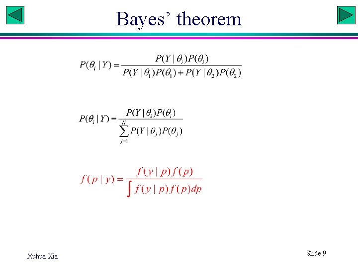
Bayes’ theorem Joint probability Marginal probability likelihood prior Marginal likelihood Bayesian inference: all based on the posterior distribution Likelihood-based inference: all based on data, and data only Statistical inference typically involves inference of parameters and the variation of their estimates Probability mass for discrete variables and probability density for continuous variables not probabi

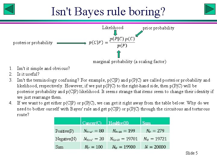
Isn't Bayes rule boring? Likelihood prior probability posterior probability marginal probability (a scaling factor) 1. Isn't it simple and obvious? 2. Is it useful? 3. Isn't the terminology confusing? For example, p(C|P) and p(P|C) are called posterior probability and likelihood, respectively. However, if we put p(P|C) to the right-hand side, then p(P|C) will be posterior probability and p(C|P) likelihood. It seems strange that items seem to change their identity if we just rearrange them. 4. If we want to get either p(C|P) or p(P|C), we can get it right away from the table below. Why do we need to bother ourself with Bayes' rule and get p(C|P) or p(P|C) through the circuitous and torturous route? Cancer(C) Healthy(H) Sum Positive(P) Negative(N) Sum Slide 5

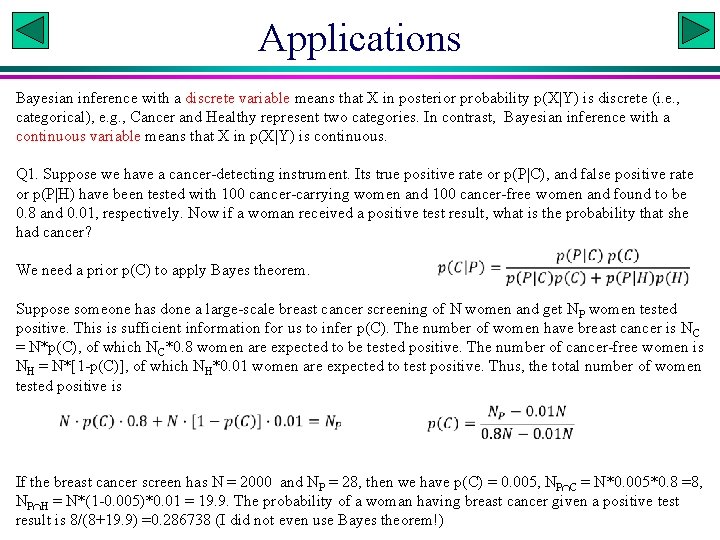
Applications Bayesian inference with a discrete variable means that X in posterior probability p(X|Y) is discrete (i. e. , categorical), e. g. , Cancer and Healthy represent two categories. In contrast, Bayesian inference with a continuous variable means that X in p(X|Y) is continuous. Q 1. Suppose we have a cancer-detecting instrument. Its true positive rate or p(P|C), and false positive rate or p(P|H) have been tested with 100 cancer-carrying women and 100 cancer-free women and found to be 0. 8 and 0. 01, respectively. Now if a woman received a positive test result, what is the probability that she had cancer? We need a prior p(C) to apply Bayes theorem. Suppose someone has done a large-scale breast cancer screening of N women and get NP women tested positive. This is sufficient information for us to infer p(C). The number of women have breast cancer is N C = N*p(C), of which NC*0. 8 women are expected to be tested positive. The number of cancer-free women is NH = N*[1 -p(C)], of which NH*0. 01 women are expected to test positive. Thus, the total number of women tested positive is If the breast cancer screen has N = 2000 and NP = 28, then we have p(C) = 0. 005, NP C = N*0. 005*0. 8 =8, NP H = N*(1 -0. 005)*0. 01 = 19. 9. The probability of a woman having breast cancer given a positive test result is 8/(8+19. 9) =0. 286738 (I did not even use Bayes theorem!)

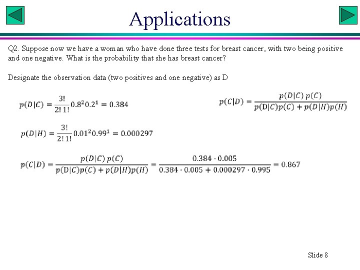
Applications Q 2. Suppose now we have a woman who have done three tests for breast cancer, with two being positive and one negative. What is the probability that she has breast cancer? Designate the observation data (two positives and one negative) as D Slide 8

Bayes’ theorem Xuhua Xia Slide 9

A simple problem • Suppose we wish to estimate the proportion of males (p) of a fish population in a large lake. • A random sample of 10 fish (N=10) includes 3 males and 7 females (M=3, F=7, N = M+F). • p = M/N is obvious, but how do we get the variance? Slide 10

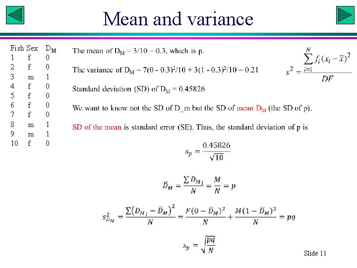
Mean and variance Fish Sex 1 f 2 f 3 m 4 f 5 f 6 f 7 f 8 m 9 m 10 f DM 0 0 1 1 0 Slide 11

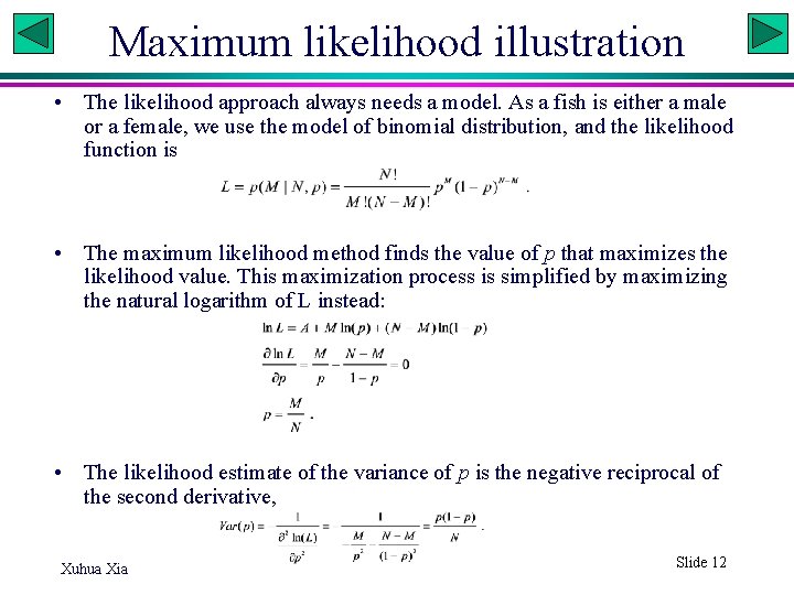
Maximum likelihood illustration • The likelihood approach always needs a model. As a fish is either a male or a female, we use the model of binomial distribution, and the likelihood function is • The maximum likelihood method finds the value of p that maximizes the likelihood value. This maximization process is simplified by maximizing the natural logarithm of L instead: • The likelihood estimate of the variance of p is the negative reciprocal of the second derivative, Xuhua Xia Slide 12

Same problem with a small sample • Suppose we wish to estimate the proportion of males (p) of a fish population in a large lake. • A random sample of 6 fish caught, all being males. • Likelihood estimate of p is p = 6/6 =1 • What is Bayesian approach to the problem? • Key concepts: all Bayesian inference is based on the posterior probability Slide 13

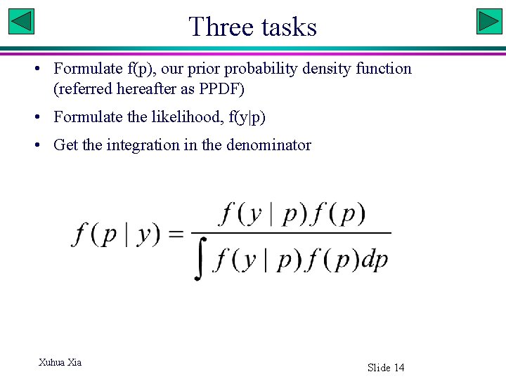
Three tasks • Formulate f(p), our prior probability density function (referred hereafter as PPDF) • Formulate the likelihood, f(y|p) • Get the integration in the denominator Xuhua Xia Slide 14

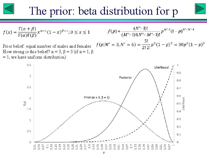
The prior: beta distribution for p Prior belief: equal number of males and females How strong is this belief? α = 3, β = 3 (if α = 1, β = 1, we have uniform distribution)

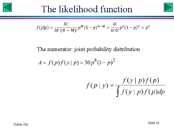
The likelihood function The numerator: joint probability distribution Xuhua Xia Slide 16

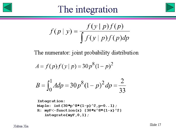
The integration The numerator: joint probability distribution Integration: Maple: int(30*p^8*(1 -p)^2, p=0. . 1); R: my. F<-function(x) {30*x^8*(1 -x)^2} integrate(my. F, 0, 1); Xuhua Xia Slide 17

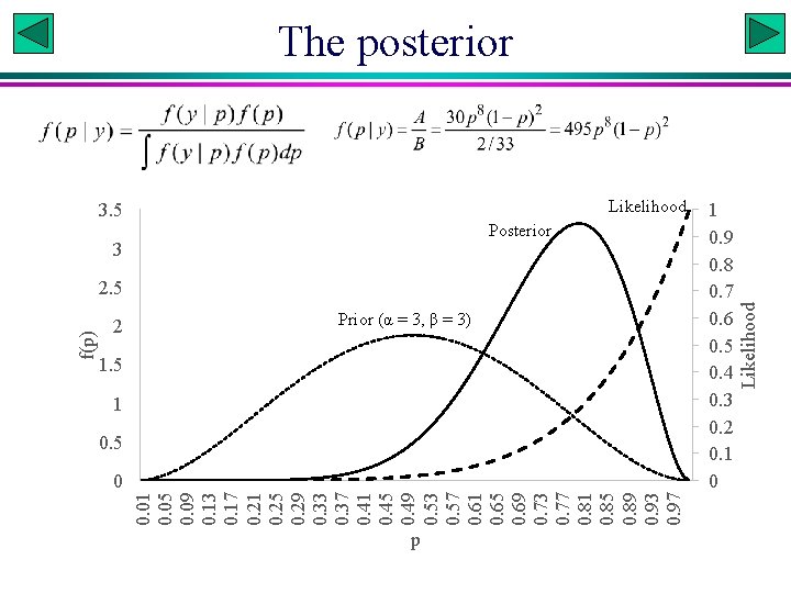
2 0. 01 0. 05 0. 09 0. 13 0. 17 0. 21 0. 25 0. 29 0. 33 0. 37 0. 41 0. 45 0. 49 0. 53 0. 57 0. 61 0. 65 0. 69 0. 73 0. 77 0. 81 0. 85 0. 89 0. 93 0. 97 f(p) 3. 5 Likelihood 3 Posterior 2. 5 Prior (α = 3, β = 3) 1. 5 1 0. 5 0 p 1 0. 9 0. 8 0. 7 0. 6 0. 5 0. 4 0. 3 0. 2 0. 1 0 Likelihood The posterior

Alternative ways to get posterior • Conjugate prior distributions (avoid the integration) • Discrete approximation (get the integration without an analytical solution) • Monte Carlo integration (get the integration without an analytical solution) • MCMC (avoid the integration) Xuhua Xia Slide 19

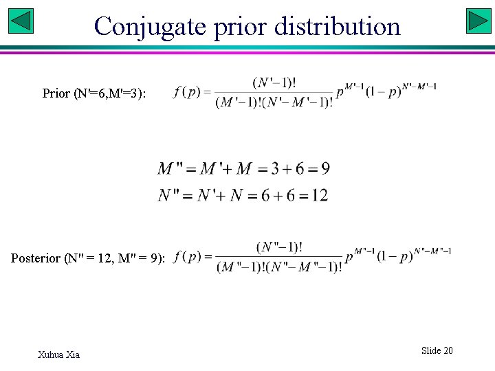
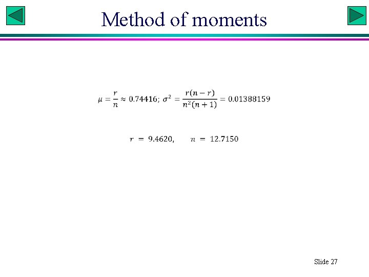
Conjugate prior distribution Prior (N'=6, M'=3): Posterior (N'' = 12, M'' = 9): Xuhua Xia Slide 20

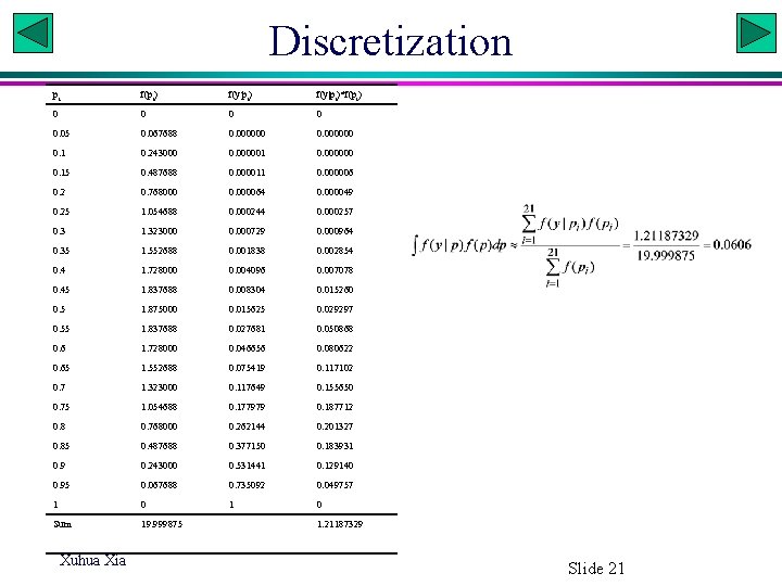
Discretization pi f(pi) f(y|pi)*f(pi) 0 0 0. 05 0. 067688 0. 000000 0. 1 0. 243000 0. 000001 0. 000000 0. 15 0. 487688 0. 000011 0. 000006 0. 2 0. 768000 0. 000064 0. 000049 0. 25 1. 054688 0. 000244 0. 000257 0. 3 1. 323000 0. 000729 0. 000964 0. 35 1. 552688 0. 001838 0. 002854 0. 4 1. 728000 0. 004096 0. 007078 0. 45 1. 837688 0. 008304 0. 015260 0. 5 1. 875000 0. 015625 0. 029297 0. 55 1. 837688 0. 027681 0. 050868 0. 6 1. 728000 0. 046656 0. 080622 0. 65 1. 552688 0. 075419 0. 117102 0. 7 1. 323000 0. 117649 0. 155650 0. 75 1. 054688 0. 177979 0. 187712 0. 8 0. 768000 0. 262144 0. 201327 0. 85 0. 487688 0. 377150 0. 183931 0. 9 0. 243000 0. 531441 0. 129140 0. 95 0. 067688 0. 735092 0. 049757 1 0 Sum 19. 999875 Xuhua Xia 1. 21187329 Slide 21

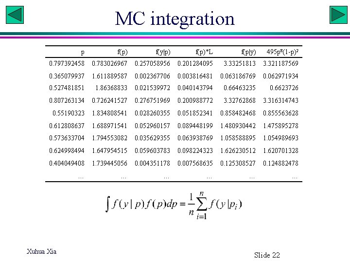
MC integration p f(p) f(y|p) f(p)*L f(p|y) 495 p 8(1 -p)2 0. 797392458 0. 783026967 0. 257058956 0. 201284095 3. 33251813 3. 321187569 0. 365079937 1. 611889587 0. 002367706 0. 003816481 0. 063186769 0. 062971934 0. 527481851 1. 86368833 0. 021539972 0. 040143794 0. 66463235 0. 6623726 0. 807263134 0. 726241527 0. 276751969 0. 200988772 3. 32762868 3. 316314743 0. 55190323 1. 834808541 0. 028260355 0. 051852341 0. 858482468 0. 855563628 0. 612808637 1. 688971541 0. 052960157 0. 089448199 1. 480930442 1. 475895278 0. 573633704 1. 794553082 0. 035629355 0. 063938769 1. 058588895 1. 054989693 0. 624998494 1. 647954515 0. 059603783 0. 098224323 1. 626230512 1. 620701328 0. 404049408 1. 739445056 0. 004351178 0. 007568635 0. 125308527 0. 124882478 … … … Xuhua Xia Slide 22

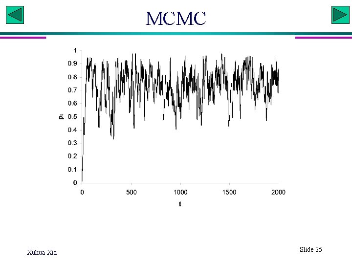
MCMC: Metropolis N <- 200000; rnd <- sample(1: 10000, N, replace=T)/10000 p <- rep(0, N) p[1] <- 0. 5 Prior_var<- 3*3/(6^2*7) for (i in seq(1: (N-1))) { p[i+1] <- rnorm(1, p[i], Prior_var) if(p[i+1]>1) { p[i+1] <- 0. 999 } else if(p[i+1]<0) { p[i+1] <- 0. 001 } fp 0 <- dbeta(p[i], 3, 3) fp 1 <- dbeta(p[i+1], 3, 3) L 0 <- p[i]^6 L 1 <- p[i+1]^6 numer <- (fp 1*L 1) denom <- (fp 0*L 0) if(numer < denom) { Alpha <- numer/denom if(rnd[i] > Alpha) { p[i+1] <- p[i] <- 0 } } } #1 chain length #2 between 0 and 1 #3 initiate a p vector #4 assign mean of the prior to p[1] #5 Eq. (23). Constrains the step size. #6 #7 propose a new p #8 #9 #10 #11 #12 #13 two prior densities fp 0 and fp 1 #14 #15 two likelihood values L 0 and L 1 #16 #17 numerator in Eq. (35) #18 denominator in Eq. (35) #19 #20 Alpha is within (0, 1). #21 #22 #23 steps to be discounted #24 #25 #26

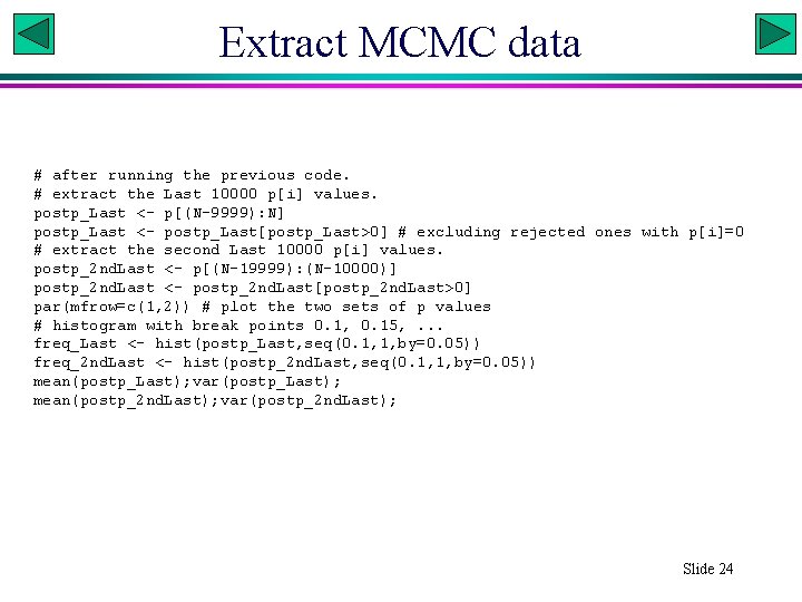
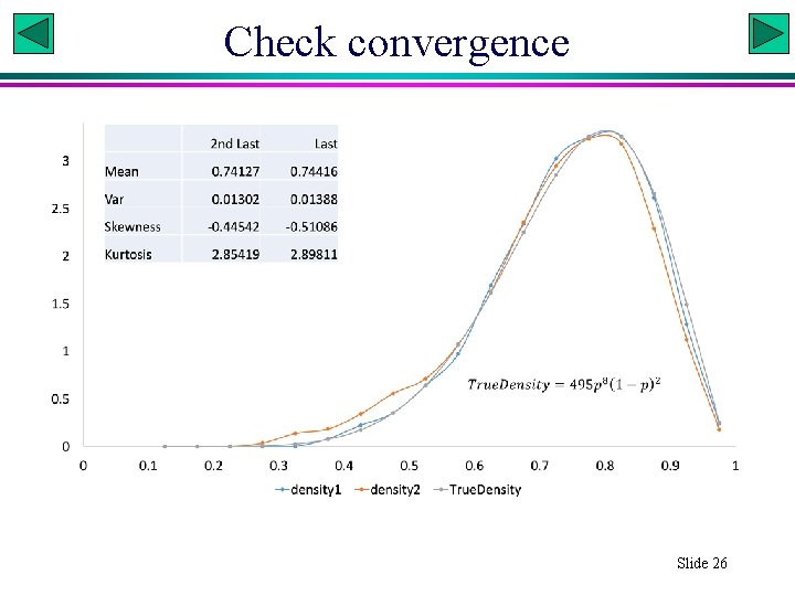
Extract MCMC data # after running the previous code. # extract the Last 10000 p[i] values. postp_Last <- p[(N-9999): N] postp_Last <- postp_Last[postp_Last>0] # excluding rejected ones with p[i]=0 # extract the second Last 10000 p[i] values. postp_2 nd. Last <- p[(N-19999): (N-10000)] postp_2 nd. Last <- postp_2 nd. Last[postp_2 nd. Last>0] par(mfrow=c(1, 2)) # plot the two sets of p values # histogram with break points 0. 1, 0. 15, . . . freq_Last <- hist(postp_Last, seq(0. 1, 1, by=0. 05)) freq_2 nd. Last <- hist(postp_2 nd. Last, seq(0. 1, 1, by=0. 05)) mean(postp_Last); var(postp_Last); mean(postp_2 nd. Last); var(postp_2 nd. Last); Slide 24

MCMC Xuhua Xia Slide 25

Check convergence Slide 26

Method of moments Slide 27

Credible & high density intervals Slide 28

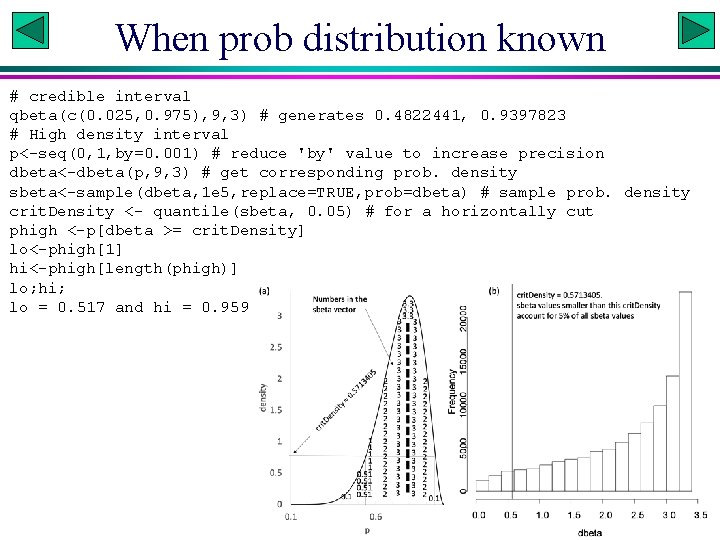
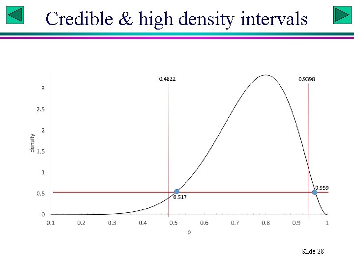
When prob distribution known # credible interval qbeta(c(0. 025, 0. 975), 9, 3) # generates 0. 4822441, 0. 9397823 # High density interval p<-seq(0, 1, by=0. 001) # reduce 'by' value to increase precision dbeta<-dbeta(p, 9, 3) # get corresponding prob. density sbeta<-sample(dbeta, 1 e 5, replace=TRUE, prob=dbeta) # sample prob. density crit. Density <- quantile(sbeta, 0. 05) # for a horizontally cut phigh <-p[dbeta >= crit. Density] lo<-phigh[1] hi<-phigh[length(phigh)] lo; hi; lo = 0. 517 and hi = 0. 959.

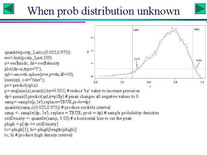
When prob distribution unknown quantile(postp_Last, c(0. 025, 0. 975)) res<-hist(postp_Last, 100) x<-res$mids; dx<-res$density plot(dx~x, type="l"); spl<-smooth. spline(x=x, y=dx, df=10); lines(spl, col="blue"); pv<-predict(spl, x) p<-seq(min(x), max(x), by=0. 001) # reduce 'by' value to increase precision dp<-pmax(0, predict(spl, x=p)$y) # pmax changes all negative values to 0. samp<-sample(p, 1 e 5, replace=TRUE, prob=dp) quantile(samp, c(0. 025, 0. 975)) # produce credible interval samp <- sample(dp, 1 e 5, replace = TRUE, prob = dp) # sample probability densities crit. Density <- quantile(samp, 0. 05) # a horizontal line to cut the peak phigh <-p[dp >= crit. Density] lo<-phigh[1]; hi<-phigh[length(phigh)] lo; hi # produce high density interval