Chapter 15 Maximum Likelihood Estimation Likelihood Ratio Test

Chapter 15 Maximum Likelihood Estimation, Likelihood Ratio Test, Bayes Estimation, and Decision Theory Chapter 15 Bei Ye, Yajing Zhao, Lin Qian, Lin Sun, Ralph Hurtado, Gao Chen, Yuanchi Xue, Tim Knapik, Yunan Min, Rui Li

Section 15. 1 Maximum Likelihood Estimation

Maximum Likelihood Estimation (MLE) 1. 2. 3. 4. Likelihood function Calculation of MLE Properties of MLE Large sample inference and delta method • 2. Calculation of Maximum Likelihood Estimation • 2. Calculation of Maximum Like

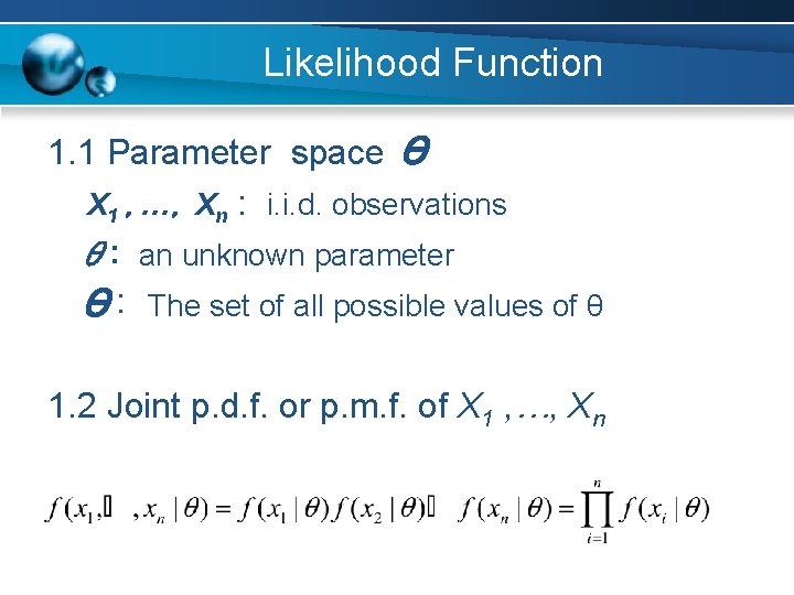
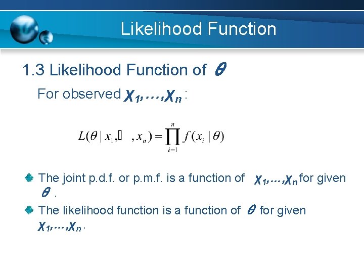
Likelihood Function 1. 1 Parameter space Θ X 1 , …, Xn : i. i. d. observations θ: an unknown parameter Θ: The set of all possible values of θ 1. 2 Joint p. d. f. or p. m. f. of X 1 , …, Xn

Likelihood Function 1. 3 Likelihood Function of θ For observed χ1, …, χn : The joint p. d. f. or p. m. f. is a function of χ1, …, χn for given θ. The likelihood function is a function of θ for given χ1, …, χn.

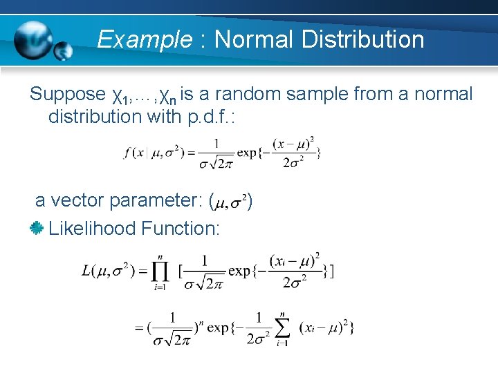
Example : Normal Distribution Suppose χ1, …, χn is a random sample from a normal distribution with p. d. f. : a vector parameter: ( Likelihood Function: )

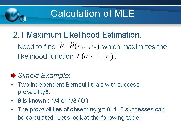
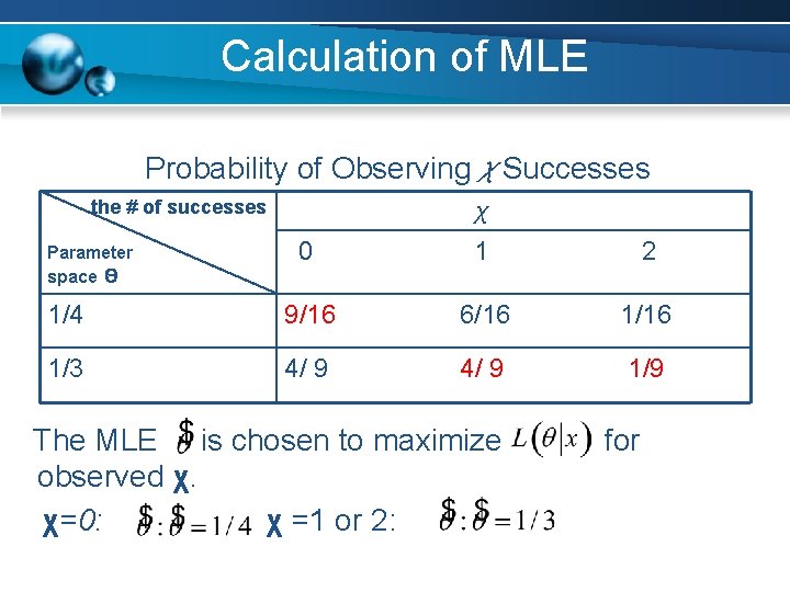
Calculation of MLE 2. 1 Maximum Likelihood Estimation: Need to find likelihood function which maximizes the . Simple Example: • Two independent Bernoulli trials with success probabilityθ. • θ is known : 1/4 or 1/3 (Θ). • The probabilities of observing χ= 0, 1, 2 successes can be calculated. Let’s look at the following table.

Calculation of MLE Probability of ObservingχSuccesses the # of successes 0 χ 1 2 1/4 9/16 6/16 1/3 4/ 9 1/9 Parameter space Θ The MLE is chosen to maximize observed χ. χ=0: χ =1 or 2: for

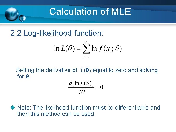
Calculation of MLE 2. 2 Log-likelihood function: Setting the derivative of L(θ) equal to zero and solving for θ. Note: The likelihood function must be differentiable and then this method can be used.

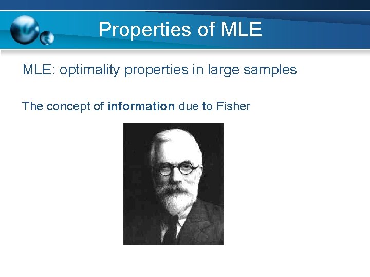
Properties of MLE: optimality properties in large samples The concept of information due to Fisher

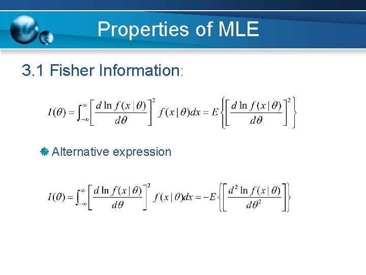
Properties of MLE 3. 1 Fisher Information: Alternative expression

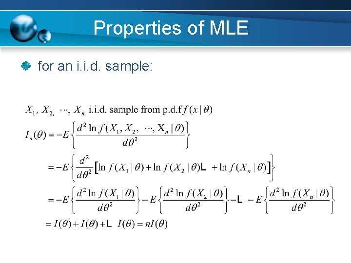
Properties of MLE for an i. i. d. sample:

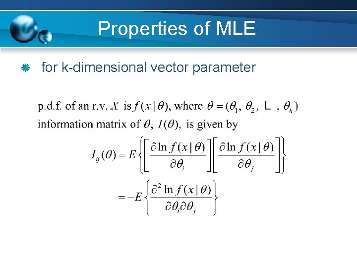
Properties of MLE for k-dimensional vector parameter

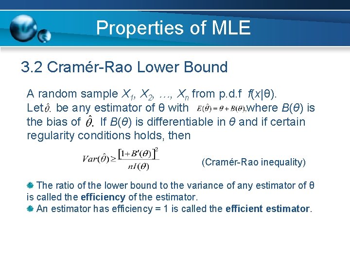
Properties of MLE 3. 2 Cramér-Rao Lower Bound A random sample X 1, X 2, …, Xn from p. d. f f(x|θ). Let be any estimator of θ with where B(θ) is the bias of If B(θ) is differentiable in θ and if certain regularity conditions holds, then (Cramér-Rao inequality) The ratio of the lower bound to the variance of any estimator of θ is called the efficiency of the estimator. An estimator has efficiency = 1 is called the efficient estimator.

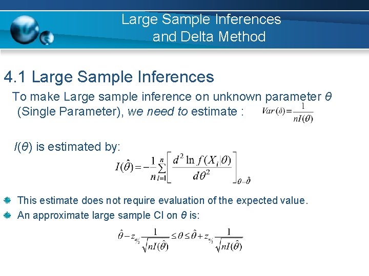
Large Sample Inferences and Delta Method 4. 1 Large Sample Inferences To make Large sample inference on unknown parameter θ (Single Parameter), we need to estimate : I(θ) is estimated by: This estimate does not require evaluation of the expected value. An approximate large sample CI on θ is:

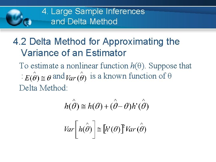
4. Large Sample Inferences and Delta Method 4. 2 Delta Method for Approximating the Variance of an Estimator To estimate a nonlinear function h(θ). Suppose that : and is a known function of θ Delta Method:

Section 15. 2 Likelihood Ratio Test

Likelihood Ratio (LR) Test 1. 2. 3. 4. Background of LR test Neyman-Pearson Lemma and Test Examples Generalized Likelihood Ratio Test

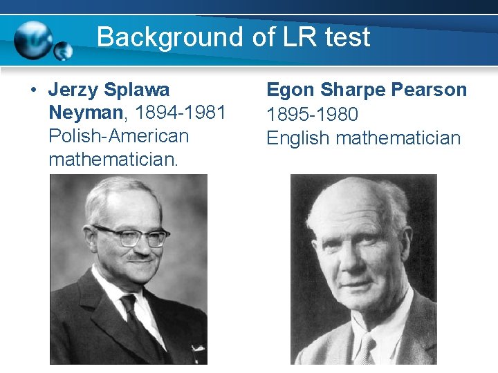
Background of LR test • Jerzy Splawa Neyman, 1894 -1981 Polish-American mathematician. Egon Sharpe Pearson 1895 -1980 English mathematician

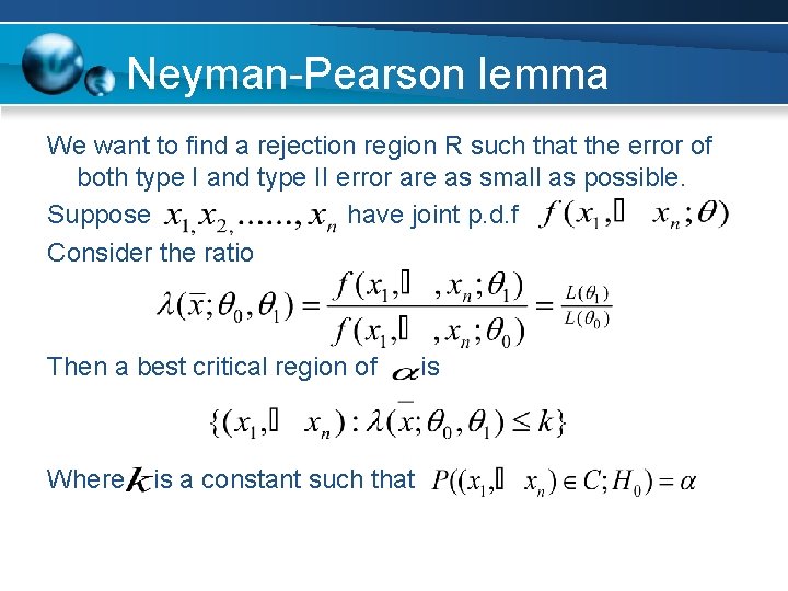
Neyman-Pearson lemma We want to find a rejection region R such that the error of both type I and type II error are as small as possible. Suppose have joint p. d. f Consider the ratio Then a best critical region of Where is a constant such that is

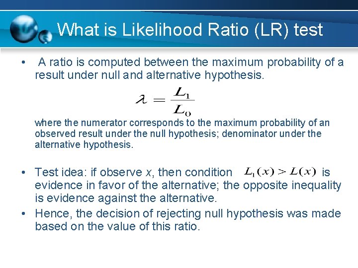
What is Likelihood Ratio (LR) test • A ratio is computed between the maximum probability of a result under null and alternative hypothesis. where the numerator corresponds to the maximum probability of an observed result under the null hypothesis; denominator under the alternative hypothesis. • Test idea: if observe x, then condition is evidence in favor of the alternative; the opposite inequality is evidence against the alternative. • Hence, the decision of rejecting null hypothesis was made based on the value of this ratio.

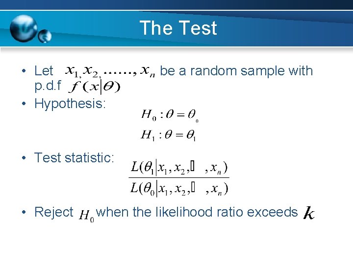
The Test • Let p. d. f • Hypothesis: be a random sample with • Test statistic: • Reject when the likelihood ratio exceeds

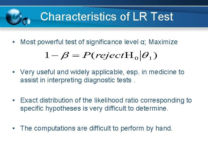
Characteristics of LR Test • Most powerful test of significance level α; Maximize • Very useful and widely applicable, esp. in medicine to assist in interpreting diagnostic tests. • Exact distribution of the likelihood ratio corresponding to specific hypotheses is very difficult to determine. • The computations are difficult to perform by hand.

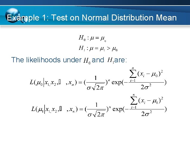
Example 1: Test on Normal Distribution Mean The likelihoods under and are:

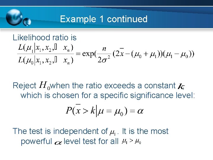
Example 1 continued Likelihood ratio is Reject when the ratio exceeds a constant , which is chosen for a specific significance level: The test is independent of. It is the most powerful level test for all.

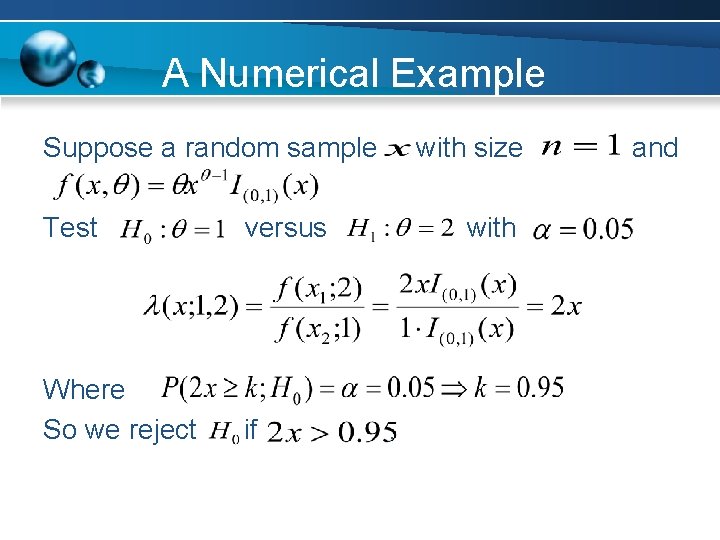
A Numerical Example Suppose a random sample Test versus Where So we reject if with size with . and

Generalized Likelihood Ratio Test • Neyman-Pearson Lemma shows that the most powerful test for a Simple vs. Simple hypothesis testing problem is a Likelihood Ratio Test. • We can generalize the likelihood ratio method for the Composite vs. Composite hypothesis testing problem.

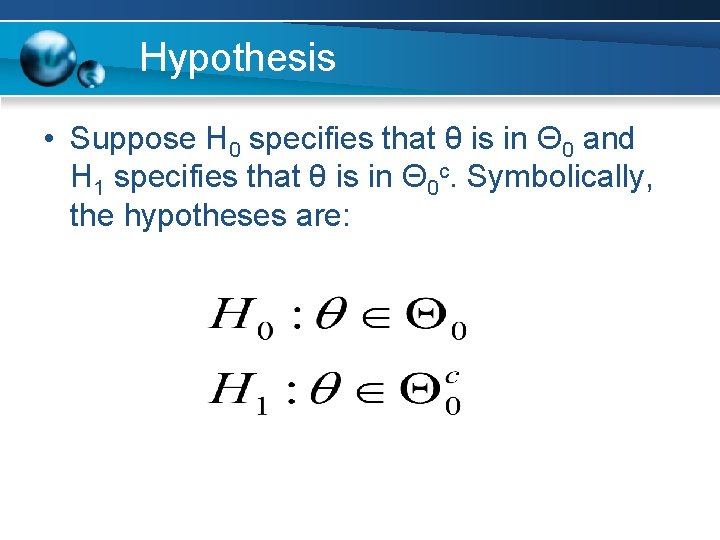
Hypothesis • Suppose H 0 specifies that θ is in Θ 0 and H 1 specifies that θ is in Θ 0 c. Symbolically, the hypotheses are:

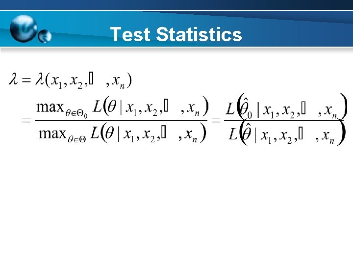
Test Statistics

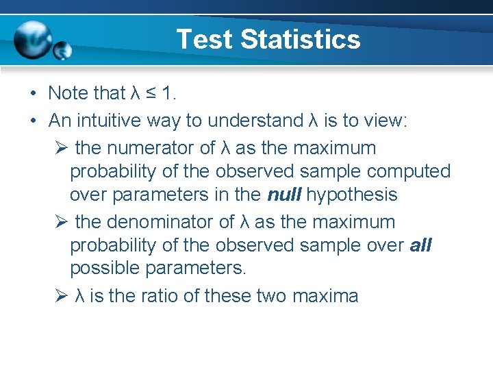
Test Statistics • Note that λ ≤ 1. • An intuitive way to understand λ is to view: Ø the numerator of λ as the maximum probability of the observed sample computed over parameters in the null hypothesis Ø the denominator of λ as the maximum probability of the observed sample over all possible parameters. Ø λ is the ratio of these two maxima

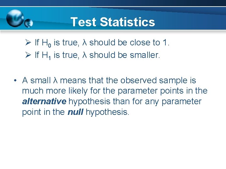
Test Statistics Ø If H 0 is true, λ should be close to 1. Ø If H 1 is true, λ should be smaller. • A small λ means that the observed sample is much more likely for the parameter points in the alternative hypothesis than for any parameter point in the null hypothesis.

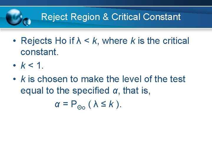
Reject Region & Critical Constant • Rejects Ho if λ < k, where k is the critical constant. • k < 1. • k is chosen to make the level of the test equal to the specified α, that is, α = PΘo ( λ ≤ k ).

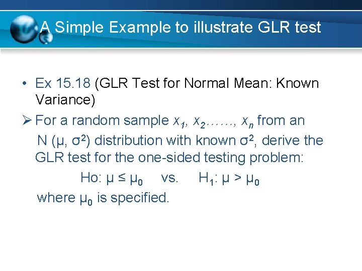
A Simple Example to illustrate GLR test • Ex 15. 18 (GLR Test for Normal Mean: Known Variance) Ø For a random sample x 1, x 2……, xn from an N (μ, σ2) distribution with known σ2, derive the GLR test for the one-sided testing problem: Ho: µ ≤ µ 0 vs. H 1: µ > µ 0 where µ 0 is specified.

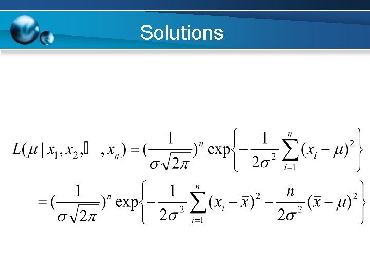
Solutions The likelihood function is

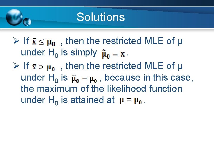
Solutions Ø If , then the restricted MLE of µ under H 0 is simply. Ø If , then the restricted MLE of µ under H 0 is , because in this case, the maximum of the likelihood function under H 0 is attained at.

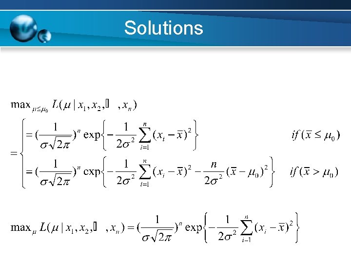
Solutions Thus, the numerator & denominator of the likelihood ratio are showing below, respectively

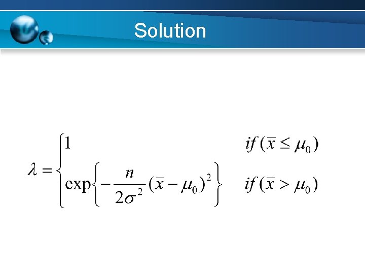
Solution Taking the ratio of the two and canceling the common terms, we get

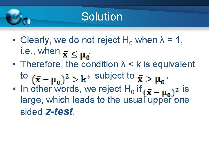
Solution • Clearly, we do not reject H 0 when λ = 1, i. e. , when. • Therefore, the condition λ < k is equivalent to subject to. • In other words, we reject H 0 if is large, which leads to the usual upper one sided z-test.

Section 15. 3 Bayesian Inference

Bayesian Inference 1. 2. 3. 4. Background of Bayesian Inference defined Bayesian Estimation Bayesian Testing

Background of Thomas Bayes • Thomas Bayes – 1702 – 1761 – British mathematician and Presbyterian minister – Fellow of the Royal Society – Studied logic and theology at the University of Edinburgh – He was barred from studying at Oxford and Cambridge because of his religion

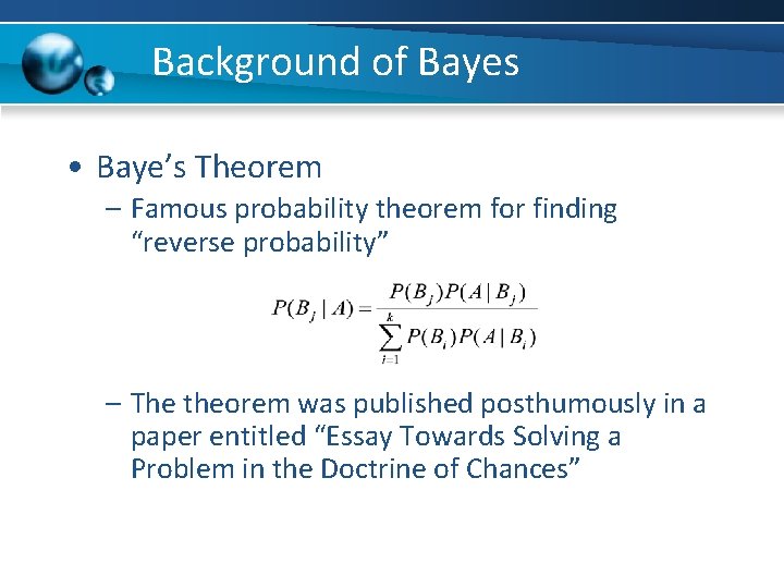
Background of Bayes • Baye’s Theorem – Famous probability theorem for finding “reverse probability” – The theorem was published posthumously in a paper entitled “Essay Towards Solving a Problem in the Doctrine of Chances”

Bayesian Inference • Application to Statistics – Qualitative Overview – Estimate an unknown parameter – Assumes the investigator has some prior knowledge of the unknown parameter – Assumes the prior knowledge can be summarized in the form of a probability distribution on , called the prior distribution – Thus, is a random variable

Bayesia • Application to Statistics – Qualitative Overview (cont. ) – The data are used to update the prior distribution and obtain the posterior distribution – Inferences on are based on the posterior distribution

Bayesian Inference • Criticisms by Frequentists – Prior knowledge is not accurate enough to form a meaningful prior distribution – Perceptions of prior knowledge differ from person to person – This may cause inferences on the same data to differ from person to person.

Some Key Terms in Bayesian Inference… In the classical approach the parameter, θ, is thought to be an unknown, but fixed, quantity. In the Bayesian approach, θ is considered to be a quantity whose variation can be described by a probability distribution which is called prior distribution. • prior distribution – a subjective distribution, based on experimenter’s belief, and is formulated before the data are seen. • posterior distribution – is computed from the prior and the likelihood function using Bayes’ theorem. • posterior mean – the mean of the posterior distribution • posterior variance – the variance of the posterior distribution • conjugate priors - a family of prior probability distributions in which the key property is that the posterior probability distribution also belongs to the family of the prior probability distribution

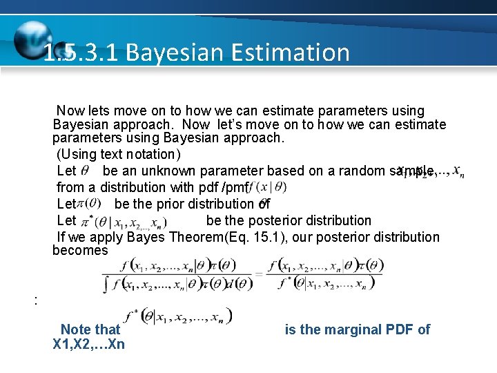
1. 5. 3. 1 Bayesian Estimation Now lets move on to how we can estimate parameters using Bayesian approach. Now let’s move on to how we can estimate parameters using Bayesian approach. (Using text notation) Let be an unknown parameter based on a random sample, from a distribution with pdf /pmf Let be the prior distribution of Let be the posterior distribution If we apply Bayes Theorem(Eq. 15. 1), our posterior distribution becomes : Note that X 1, X 2, …Xn is the marginal PDF of

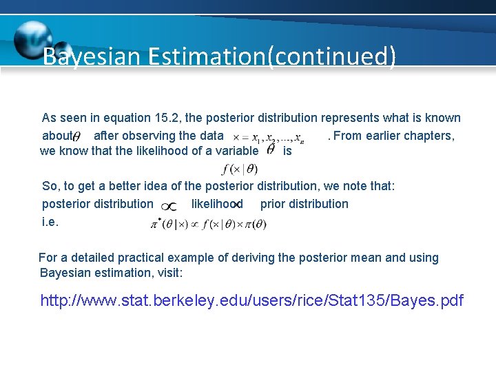
Bayesian Estimation(continued) As seen in equation 15. 2, the posterior distribution represents what is known about after observing the data. From earlier chapters, we know that the likelihood of a variable is So, to get a better idea of the posterior distribution, we note that: posterior distribution likelihood prior distribution i. e. For a detailed practical example of deriving the posterior mean and using Bayesian estimation, visit: http: //www. stat. berkeley. edu/users/rice/Stat 135/Bayes. pdf

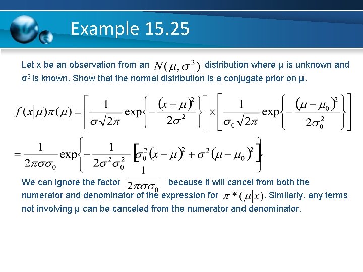
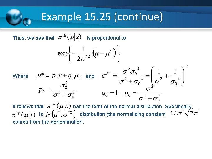
Example 15. 25 Let x be an observation from an distribution where μ is unknown and σ2 is known. Show that the normal distribution is a conjugate prior on μ. We can ignore the factor because it will cancel from both the numerator and denominator of the expression for. Similarly, any terms not involving μ can be canceled from the numerator and denominator.

Example 15. 25 (continue) Thus, we see that is proportional to Where and It follows that has the form of the normal distribution. Specifically, is distribution (the normalizing constant comes from the denomination.

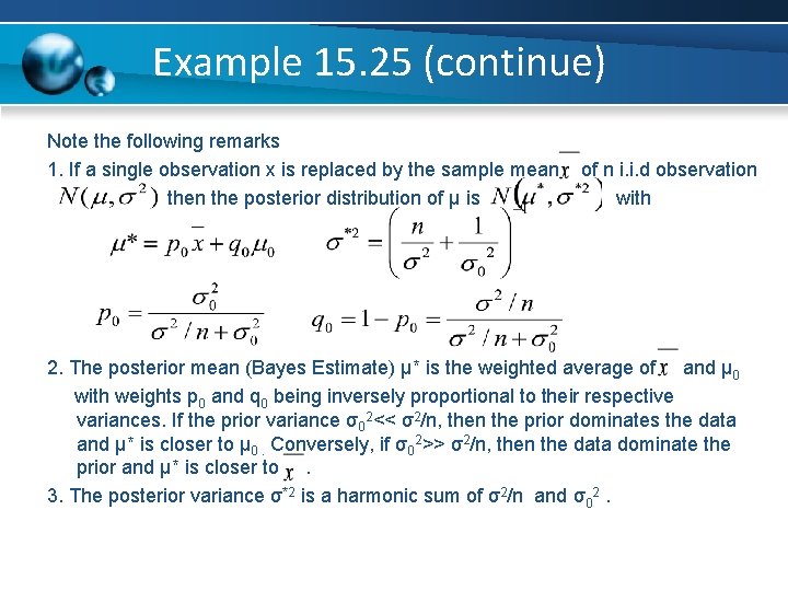
Example 15. 25 (continue) Note the following remarks 1. If a single observation x is replaced by the sample mean the posterior distribution of μ is of n i. i. d observation with 2. The posterior mean (Bayes Estimate) μ* is the weighted average of and μ 0 with weights p 0 and q 0 being inversely proportional to their respective variances. If the prior variance σ02<< σ2/n, then the prior dominates the data and μ* is closer to μ 0. Conversely, if σ02>> σ2/n, then the data dominate the prior and μ* is closer to. 3. The posterior variance σ*2 is a harmonic sum of σ2/n and σ02.

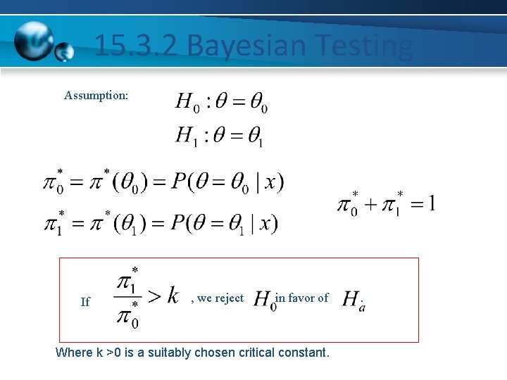
15. 3. 2 Bayesian Testing Assumption: If , we reject in favor of Where k >0 is a suitably chosen critical constant. .

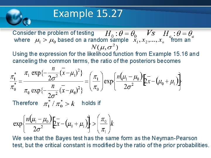
Example 15. 27 Consider the problem of testing where based on a random sample from an Using the expression for the likelihood function from Example 15. 16 and canceling the common terms, the ratio of the posteriors becomes Therefore holds if We see that the Bayes test has the same form as the Neyman-Pearson test, but the critical constant is modified by the ratio of the prior probabilities.

Decision theory 1. Definition – Loss – Risk 2. Comparison of estimators – Admissibility – Minimax – Bayes risk 3. Example of hypothesis testing

Section 15. 4 Decision Theory

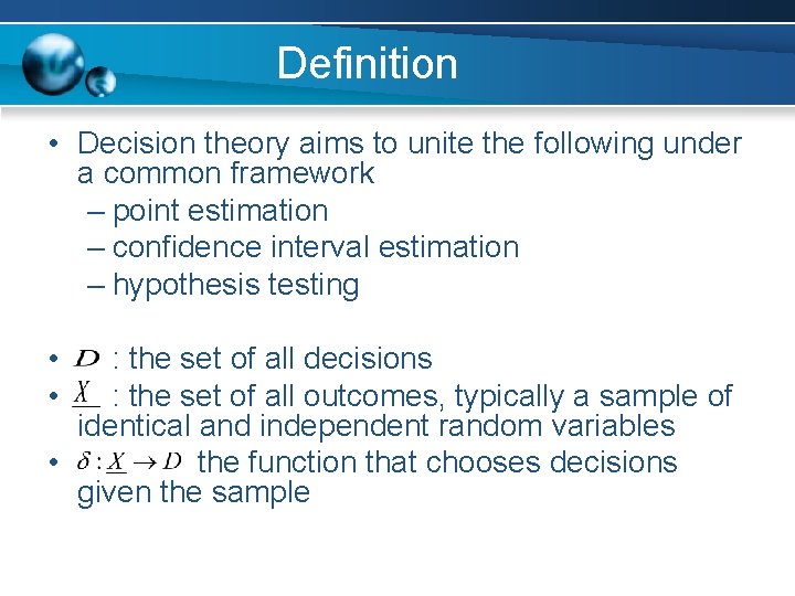
Definition • Decision theory aims to unite the following under a common framework – point estimation – confidence interval estimation – hypothesis testing • • : the set of all decisions : the set of all outcomes, typically a sample of identical and independent random variables • the function that chooses decisions given the sample

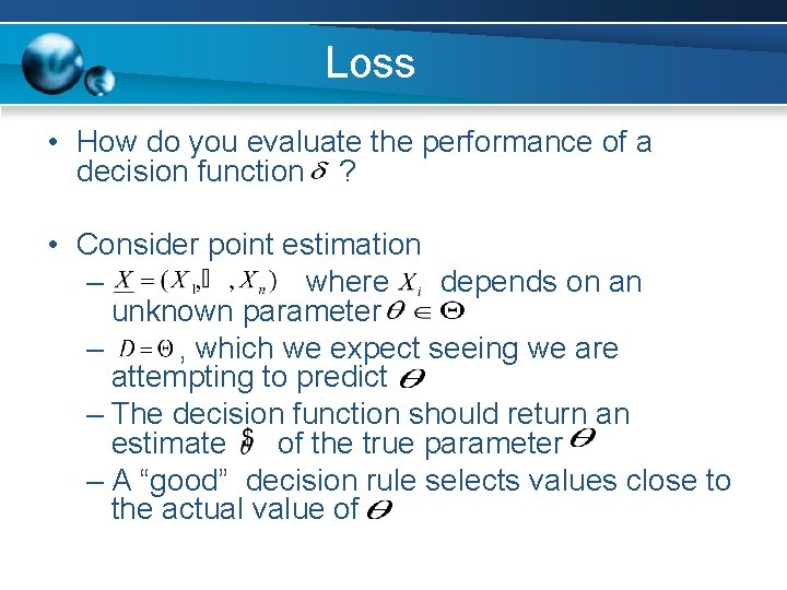
Loss • How do you evaluate the performance of a decision function ? • Consider point estimation – where depends on an unknown parameter – , which we expect seeing we are attempting to predict – The decision function should return an estimate of the true parameter – A “good” decision rule selects values close to the actual value of

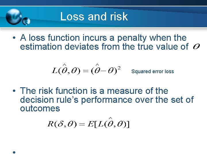
Loss and risk • A loss function incurs a penalty when the estimation deviates from the true value of Squared error loss • The risk function is a measure of the decision rule’s performance over the set of outcomes

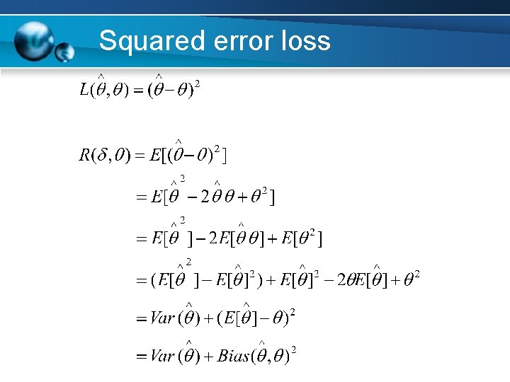
Squared error loss

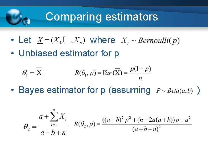
Comparing estimators • Let where • Unbiased estimator for p • Bayes estimator for p (assuming )

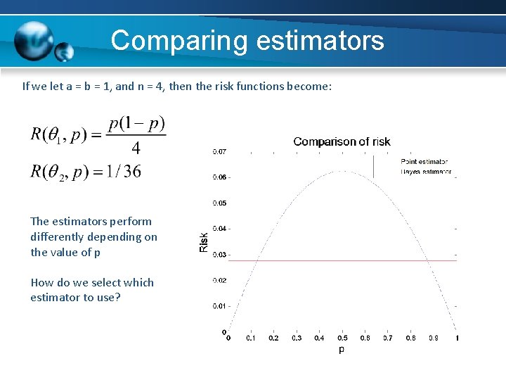
Comparing estimators If we let a = b = 1, and n = 4, then the risk functions become: The estimators perform differently depending on the value of p How do we select which estimator to use?

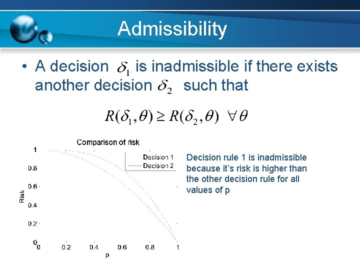
Admissibility • A decision is inadmissible if there exists another decision such that Decision rule 1 is inadmissible because it’s risk is higher than the other decision rule for all values of p

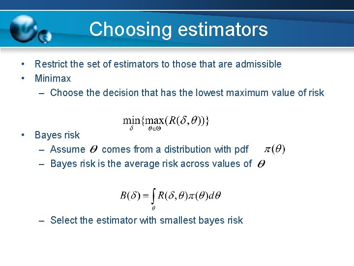
Choosing estimators • Restrict the set of estimators to those that are admissible • Minimax – Choose the decision that has the lowest maximum value of risk • Bayes risk – Assume comes from a distribution with pdf – Bayes risk is the average risk across values of – Select the estimator with smallest bayes risk

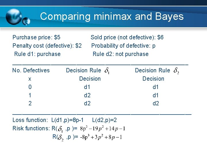
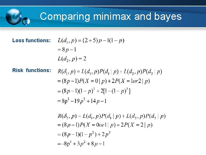
Comparing minimax and Bayes Purchase price: $5 Sold price (not defective): $6 Penalty cost (defective): $2 Probability of defective: p Rule d 1: purchase Rule d 2: not purchase ____________________________ No. Defectives Decision Rule x Decision 0 d 1 1 d 2 d 1 2 d 2 ____________________________ Loss function: L(d 1, p)=8 p-1 L(d 2, p)=2 Risk functions: R( , p )=

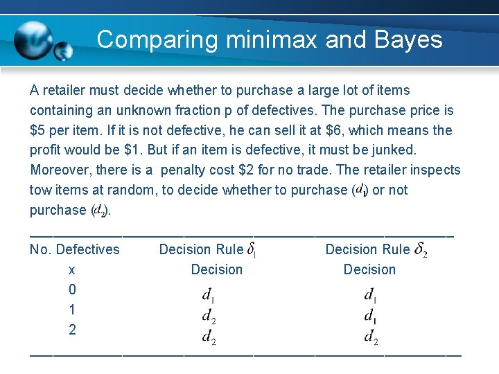
Comparing minimax and Bayes A retailer must decide whether to purchase a large lot of items containing an unknown fraction p of defectives. The purchase price is $5 per item. If it is not defective, he can sell it at $6, which means the profit would be $1. But if an item is defective, it must be junked. Moreover, there is a penalty cost $2 for no trade. The retailer inspects tow items at random, to decide whether to purchase ( ) or not purchase ( ). ____________________________ No. Defectives Decision Rule x Decision 0 1 2 ____________________________

Comparing minimax and bayes Loss functions: Risk functions:

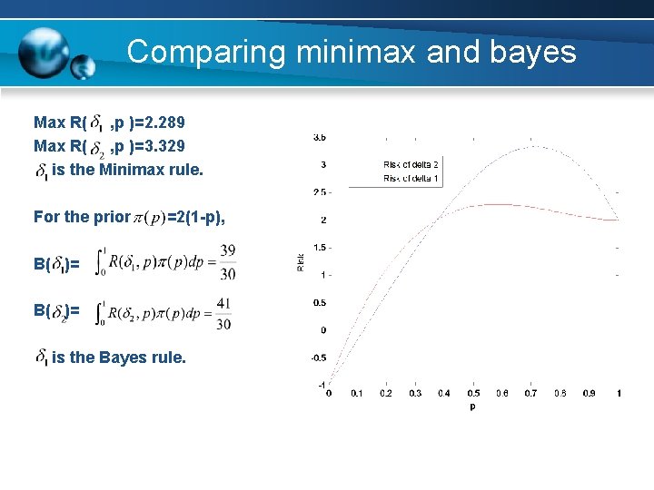
Comparing minimax and bayes Max R( , p )=2. 289 Max R( , p )=3. 329 is the Minimax rule. For the prior =2(1 -p), B( )= is the Bayes rule.

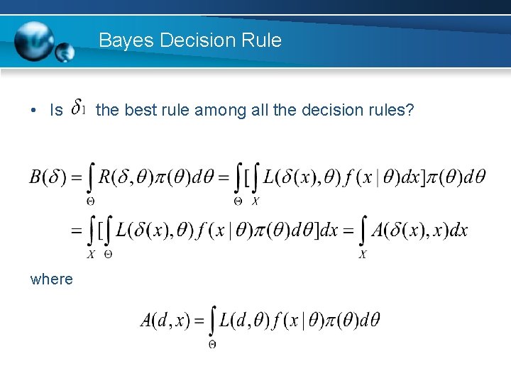
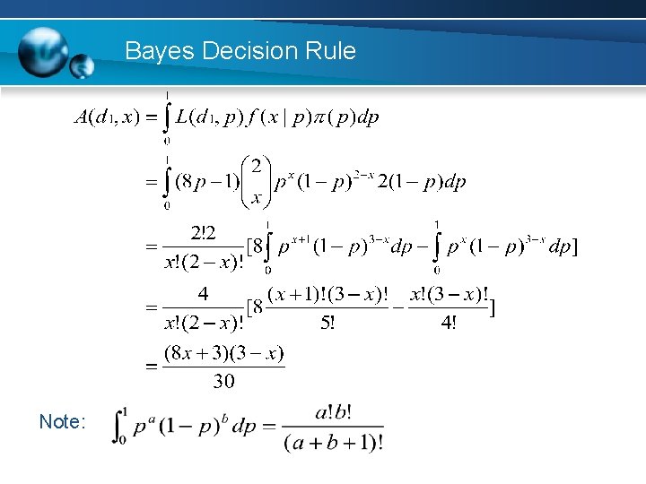
Bayes Decision Rule • Is where the best rule among all the decision rules?

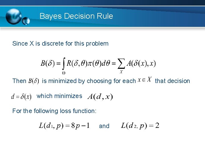
Bayes Decision Rule Since X is discrete for this problem Then is minimized by choosing for each which minimizes For the following loss function: and that decision

Bayes Decision Rule Note:

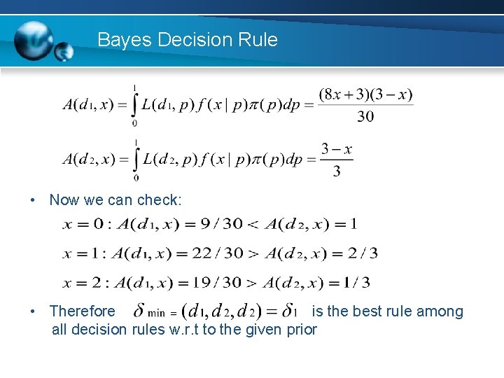
Bayes Decision Rule • Now we can check: • Therefore is the best rule among all decision rules w. r. t to the given prior

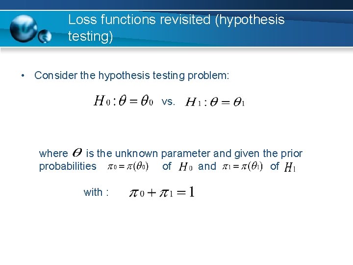
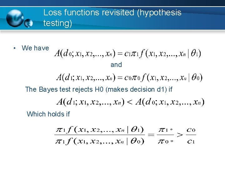
Loss functions revisited (hypothesis testing) • Consider the hypothesis testing problem: vs. where is the unknown parameter and given the prior probabilities of and of with :

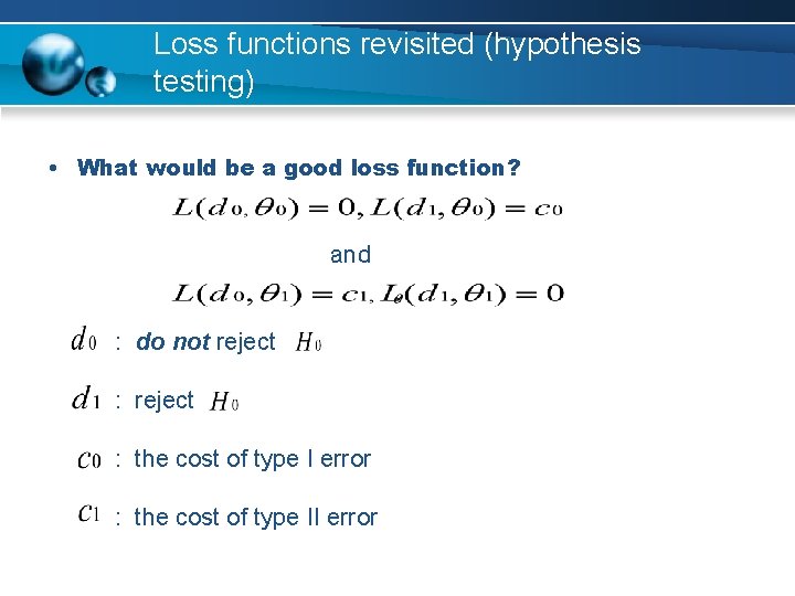
Loss functions revisited (hypothesis testing) • What would be a good loss function? and : do not reject : the cost of type I error : the cost of type II error

Loss functions revisited (hypothesis testing) • We have and The Bayes test rejects H 0 (makes decision d 1) if Which holds if

Trendy ending slide