Hidden Markov Models Jacques van Helden AixMarseille Universit
 Lab. Theory and Approaches of")


")


 n n Transition frequencies for a Markov model of order")
 n n Transition frequencies for a Markov model of order")
 n n Transition frequencies for a Markov model of order")


")


")


 are an extension of")


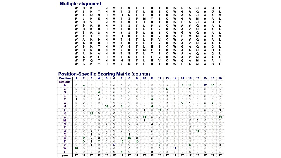
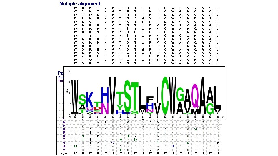
 n Starting from a multiple alignment, one can")


 q q")


")
")
- Slides: 46
Hidden Markov Models Jacques van Helden Aix-Marseille Université (AMU) Lab. Theory and Approaches of Genomic Complexity (TAGC) https: //tagc. univ-amu. fr/ Institut Français de Bioinformatique (IFB) http: //www. france-bioinformatique. fr Jacques. van. Helden@france-bioinformatique. fr https: //orcid. org/0000 -0002 -8799 -8584
A seminal book n n In 1998, Richard Durbin, Sean Eddy, A. Krogh and G. Mitchison published a seminal book entitled « Biological sequence analysis » q A tutorial introduction to hidden Markov models and other probabilistic modelling approaches in computational sequence analysis. q The authors restate the classical sequence analysis problems in terms of Hidden Markov Models (HMM). q Even their table of contents is presented as an HMM (their Figure 1. 1 below) Biological Sequence Analysis: Probabilistic Models of Proteins and Nucleic Acids. Richard Durbin, Sean Eddy, Anders Krogh, and Graeme Mitchison. Cambridge University Press, 1998. ISBN 0 -521 -62041 -4 (hardback)
Applications of Hidden Markov Models in biology n n n Hidden Markov models can be applied to solve a diversity of problems in bioinformatics Sequence segmentation q Detection of Cp. G islands q Intron/exon prediction Motif detection q Protein domains (long motifs in peptidic sequences) q Transcription factor binding sites (short motifs on DNA sequences) Secondary structure prediction …
Markov models (nothing to hide so far)
Markov process n n n A Markov process is defined by q A finite number of states (A, B, C, …) Example: 2 -state Markov process q States: {X, Y} Transitions: q {X X, X Y, Y X, X Y} The probability of transition from each state to each other one is described in a transition matrix. q Rows: current state si q Columns: next state si+1 q Values P(si+1 | si ) q Transition probabilities sum to 1 on each row Examples of Markov models to annotate genomic sequences 1. State X = intron, State Y = exon 2. State X = transcribed region, state Y = intergenic region 3. State X = Cp. G island; State Y = other genomic region 2 -states Markov process X Y Transition matrix X Y X 0. 9 0. 1 Y 0. 2 0. 8 Examples of biological applications 1. Segmentation of the genome into transcribed and intergenic regions Genome fragment transcript 2. Segmentation of transcribed regions into introns and exons intron exon 3. Segmentation of the genome into Cp. G islands and non-Cp. G islands Cp. G island non-Cp. G island
Markov process n In order to annotate the genome, we could conceive a multi- k-states Markov process state markov model that would represent the different 1. State W = intron, 2. State X = exon W 3. State Y = Cp. G island; 4. State Z = other genomic region X E B Y Z Segmentation of the genome into different types of regions intron exon Cp. G island other type of genomic region Transition matrix (arbitrary values) W X Y Z W 0. 990 0. 010 0. 000 X 0. 010 0. 988 0. 001 Y 0. 00000 0. 00002 0. 99898 0. 00100 Z 0 0. 000002 0. 000001 0. 999997
Markov model of a sequence n n We can model a macromolecular sequence as a Markov process q DNA : n = 4 states (A, C, G, T) q Proteins: n = 20 states (amino acids) q Optionally, additional states can be used to represent the beginning (B) of and the end (E) of the sequence. This enables to generate sequences of different lengths. Transition probabilities indicate the probability to generate a given residue (suffix) given the current residue (prefix) 4 -states Markov process for DNA sequence A B E G n Exercise q DNA sequences are generated using a Markov model with ending probability of 0. 99 (irrespective of the current residue). What is the distribution of sequence lengths? C T
Probability of a sequence segment n n What is the probability for a given sequence segment ? Different models can be chosen q Bernoulli model • Assumes independence between successive nucleotides. • The probability of each residue is fixed a priori (prior residue probability) n Example: P(A) = 0. 35; P(T) = 0. 32; P(C) = 0. 17; P(G) = 0. 16 • Particular case: equiprobable residues n P(A) = P(T) = P(C) = P(G) = 0. 25 n Simple, but NOT realistic ! q Markov model • The probability of each residue depends on the m preceding residues. • The parameter m is called the order of the Markov model • Remark: a Bernoulli model can be considered as a Markov model of order 0 8
Independent and equiprobable nucleotides n n n The simplest model : Bernoulli with identically and independently (i. i. d. ) distributed nucleotides. p = P(A) = P(C) = P(G) = P(T)= 0. 25 The probability of a sequence q Is the product of its residue probabilities (independence) q Equiprobability: since all residues have the same probability, it is simply computed as the residue proba (p) to the power of the sequence length (L) • S is a sequence segment (e. g. an oligonucleotide) • L length of the sequence segment • p nucleotide probability • P(S) is the probability to observe this sequence segment at given position of a larger sequence Example q P(CACGTG) = 0. 256 = 2. 44 e-4 9
Bernoulli model : independently distributed nucleotides A more refined model consists in using residuespecific probabilities. The probability of each residue is assumed to be constant on the whole sequence (Bernoulli schema). n The probability of a sequence is the product of its residue probabilities. q i = 1. . k is the index of nucleotide positions q ri is the residue found at position I q P(ri) is the probability of this residue n Example: non-coding sequences in the yeast genome q P(A) = P(T) = 0. 325 q P(C) = P(G) = 0. 175 q P(CACGTG) = P(C) P(A) P(C) P(G) P(T) P(G) = 0. 3254 * 0. 1752 = 9. 91 E-5 n 10
Bernoulli models n A Bernoulli model assumes that q q n n each residue has a specific prior probability this probability is constant over the sequence (no context dependencies) The heat-maps below depict the nucleotide frequencies in non-coding upstream sequences of various organisms. The frequencies of AT versus CG show strong inter-organism differences. Saccharomyces cerevisiae (Fungus) Escherichia coli K 12 (Proteobacteria) Mycoplasma genitalium (Firmicute, intracellular) Bacillus subtilis (Firmicute, extracellular) Plasmodium falciparum (Aplicomplexa, intracellular) Anopheles gambiae (Insect) Mycobacterium leprae (Actinobacteria) Homo sapiens (Mammalian) 11
Markov chains and transition matrices In a Markov model, the probability to find a letter at position i depends on the residues found at the m preceding residues. n The tables represent the transition matrices for Markov chain models of order m=1 (top) and m=2 (bottom). n Each row specifies one prefix, each column one suffix. n The values indicate the probability to observe a given residue (suffix ri) at position (i) of the sequence, as a function of the m preceding residues (the prefix Si-m, i-1) n Particular case q A Bernoulli model is a Markov model of order 0. n 12
Markov model estimation (“training”) n n Transition frequencies for a Markov model of order m can be estimated from the frequencies observed for oligomers (k-mers) of length k=m+1 in a reference sequence set. Example q The upper table shows dinucleotide frequencies (k=2) computed from the whole set of upstream sequences of the yeast Saccharomyces cerevisiae. q This table can be used to estimate a Markov model of order m = k– 1 = 1. 13
Markov model estimation (“training”) n n Transition frequencies for a Markov model of order m can be estimated from the frequencies observed for oligomers (k-mers) of length k=m+1 in a reference sequence set. Example q The upper table shows dinucleotide frequencies (k=2) computed from the whole set of upstream sequences of the yeast Saccharomyces cerevisiae. q This table can be used to estimate a Markov model of order m = k– 1 = 1. Exercise: estimate P(G|T) from the dinucleotide frequency table - Give the formula with symbols - Replace the symbols by their values - Compute the result 14
Markov model estimation (“training”) n n Transition frequencies for a Markov model of order m can be estimated from the frequencies observed for oligomers (k-mers) of length k=m+1 in a reference sequence set. Example q The upper table shows dinucleotide frequencies (k=2) computed from the whole set of upstream sequences of the yeast Saccharomyces cerevisiae. q This table can be used to estimate a Markov model of order m = k– 1 = 1. 15
Examples of transition matrices n n n The two tables below show the transition matrices for a Markov model of order 1 (top) and 2 (bottom), respectively. Trained with the whole set of non-coding upstream sequences of the yeast Saccharomyces cerevisiae. Notice the high probability of transitions from AA to A and TT to T. Pre/Suffix A C G T a 0. 371 0. 165 0. 178 0. 285 P(Prefix) 0. 321 c 0. 327 0. 190 0. 167 0. 316 0. 183 g 0. 312 0. 214 0. 189 0. 285 0. 177 0. 320 t 0. 273 0. 179 0. 173 0. 375 Sym 1. 283 0. 748 0. 708 1. 261 P(suffix) 0. 321 0. 183 0. 176 0. 320 Prefix/Suffix A C aa 0. 416 0. 151 0. 187 0. 246 0. 119 ac 0. 352 0. 181 0. 171 0. 297 0. 053 ag 0. 339 0. 202 0. 193 0. 267 0. 057 at 0. 346 0. 162 0. 326 0. 092 ca 0. 344 0. 185 0. 180 0. 291 0. 060 cc 0. 305 0. 200 0. 171 0. 324 0. 035 cg 0. 282 0. 232 0. 193 0. 294 0. 031 ct 0. 241 0. 189 0. 184 0. 385 0. 058 ga 0. 411 0. 144 0. 187 0. 257 0. 055 gc 0. 334 0. 192 0. 182 0. 293 0. 038 gg 0. 315 0. 220 0. 194 0. 271 0. 033 gt 0. 307 0. 156 0. 200 0. 338 0. 050 ta 0. 304 0. 184 0. 160 0. 352 0. 087 tc 0. 313 0. 192 0. 152 0. 343 0. 057 tg 0. 300 0. 214 0. 180 0. 307 0. 055 tt Sum 0. 218 0. 194 0. 164 0. 423 0. 120 5. 127 3. 000 2. 860 5. 013 0. 321 0. 183 0. 176 0. 319 P(suffix) G T P(Prefix) 16
Markov chains and Bernoulli models n n By extension of the concept of Markov chain, Bernoulli models can be qualified as Markov models of order 0 (the order 0 means that there is no dependency between a residue and the preceding ones). The prior probabilities of a Makov model of order m=0 can be estimated from the residue of single nucleotides (k=m+1=1) in a background sequence set. The table below shows the residue frequencies in the genomes of the yeast Saccharomyces cerevisiae and the bacteria Escherichia coli K 12, respectively. Notice the strong differences between these genomes. 17
Scoring a sequence segment with a Markov model n Exercise: compute the probability P(S|B) of a sequence segment S with a background Markov model B of order 2, estimated from 3 nt frequencies on the yeast non-coding upstream sequences. CCTACTATATGCCCAGAATT Sequence probability given the background model B 18
Scoring a sequence segment with a Markov model n The example below illustrates the computation of the probability P(S|B) of a sequence segment S with a background Markov model B of order 2, estimated from 3 nt frequencies on the yeast non-coding upstream sequences. CCTACTATATGCCCAGAATT Background model B Sequence probability given the backgound model 19
Sequence discrimination
Discriminating sequences based on alternative Markov models n Cp. G islands Genomic background Log-odds transition matrix
Exercise 1. Open a connection to the UCSC genome browser, and select the table browser tool. 2. Choose a mammalian genome (e. g. Human version hg 38), select Cp. G track in the Regulation group, and download the sequences of all the annotated Cp. G islands. 3. Open a connection to RSAT Metazoa 4. Compute the transition matrix of a 1 st order Markov the tool create background model. 5. Use the tool random genome fragments to extract sequences of random genomic fragments of the same sizes as the Cp. G island. 6. Use these random genome fragments to compute the genomic background (transition matrix of a 1 st order Markov model) 7. With the tool sequence proba, compute the sequence probabilities for each sequence file (Cp. G islands, random genome fragments) with each model (Cp. G island, genome background). 8. Open the 4 results files with R or in a spreadsheet, and compute the log-likelihood ratio log(P(S|Cp. G) / P(S|Bg)) for q q the Cp. G islands the genomic background 9. Compare the distributions of these LLR (you can depict them with histograms, boxplots, violin plots, …).
Hidden Markov Models (HMM)
Probabilities of transition between states Let us consider the genome as a Markov chain composed of a succession of regions in states Cp. G (+) or non-Cp. G islands (-) n The total size of the Human genome is 3 GB, and its annotation contain 31, 144 Cp. G islands totaling 24. 2 MB. n Exercise: based on these numbers, estimate the transition probabilities between states. n Segmentation of the genome into Cp. G islands and non-Cp. G islands Cp. G island non-Cp. G island 2 -states Markov process Cp. G (+) other (-) Transition matrix Cp. G Other
Solution: transition probabilities between states n Segmentation of the genome into Cp. G islands and non-Cp. G islands Cp. G island non-Cp. G island 2 -states Markov process Cp. G (+) other (-) Transition matrix Cp. G (+) Other (-) Cp. G (+) 0. 99871 0. 00129 Other (-) 0. 00001 0. 99999
Hidden Markov Models n n n Hidden Markov Models (HMM) are an extension of Markov chains, where we assume a process with a given number of states, and a specific probability of emitting symbols associated to each state. The state-specific emission probabilities can themselves be modeled as Markov chains, or as Bernoulli models. Example: Cp. G islands in genomic sequences q 2 states: Cp. G islands and genomic background q Each state has a specific nucleotide transition matrix q Note: the emission probabilities were computed from a random selection of genomic region, which might include some fragments of Cp. G islands. However the proportion is likely to be very low, so we can use it as estimator for the emission probabilities of non-Cp. G islands (other). Transition matrix Cp. G (+) Other (-) Cp. G (+) 0. 99871 0. 00129 Other (-) 0. 00001 0. 99999 Segmentation of the genome into Cp. G islands and non-Cp. G islands Cp. G island 2 -states Markov process Cp. G (+) non-Cp. G island Other (-) Emission probabilities Cp. G state (+) Cp. G islands Bg state Genomic background (-)
Sequence segmentation
Sequence segmentation n n Problem: given a long unannotated sequence, identify the segments corresponding to Cp. G islands. Notes q This problem differs from the discrimination problem seen before, where we assign a class to each sequence as a whole. q No unequivocal correspondence from symbols to states: the same symbol can be emitted by different state. q The state underlying each emission (nucleotide) is thus “hidden”. q We need to discover it by finding the chain of states most likely to have produced the sequence. Sequence position Cp. G island n n n Example: sequence ATTATGGGCGCGAA Each nucleotide (symbol) can be generated by either the Cp. G (upper row) or the non-Cp. G (lower row) state. Between each pair of nucleotides, we can either stay on the current state (horizontal arrows) or switch to the other state (oblique arrows) The problem amounts to find, among all possible paths from B (sequence beginning) to E (end), the path having the maximal likelihood. Exercise: how many possible paths are there between B and E? 1 2 3 4 5 6 7 8 9 10 11 12 13 14 A T T A T G G G C G A A B non-Cp. G Hidden state E A T T A T G G G C G A A ? ? ? ?
Uncovering the hidden chain of states n n In the drawing below, we highlighted one of the possible paths from the beginning to the end of the sequence ATTATGGGCGCGAA. Exercise q Annotate the sequence of hidden states with + and q Compute the probability of this path according to the previously defined parameters q How many possible paths are there between B and E? q Which path would you intuitively propose as the best? q Which path would you intuitively propose as the worse? q Compute the probability of these paths Sequence position Cp. G island Cp. G (+) Other (-) Cp. G (+) 0. 99871 0. 00129 Other (-) 0. 00001 0. 99999 Cp. G (+) Non-Cp. G (-) 1 2 3 4 5 6 7 8 9 10 11 12 13 14 A T T A T G G G C G A A B non-Cp. G Hidden state E A T T A T G G G C G A A ? ? ? ?
Viterbi algorithm n n Viterbi algorithm enables to find the optimal path in a Hidden Markov Model Same principle as dynamical programing: q Compute the probability to reach node (emitted symbol in a given state), from each one of the incoming arrows. q Assign to this node the highest of probability value, and keep track of the corresponding incoming arrow. Sequence position Cp. G island 1 2 3 4 5 6 7 8 9 10 11 12 13 14 A T T A T G G G C G A A B non-Cp. G Hidden state E A T T A T G G G C G A A ? ? ? ?
Bioinformatics Sequence motifs
Profile matrices (=position-specific scoring matrices, PSSM) n Starting from a multiple alignment, one can build a matrix which reflects the most representative residues at each position q q q Each column represents a position Each row represents a residue (20 rows for proteins, 4 rows for DNA) The cells indicate the frequency of each residue at each position of the multiple alignment.
Weight matrix
Scoring a sequence with a profile matrix
Scoring a sequence with a profile matrix
Scoring a sequence with a profile matrix
PSI-BLAST n PSI-BLAST stands for Position-Specific Iterated BLAST (Altschul et al, 1997) q q n BLAST runs a first time in normal mode. Resulting sequences are aligned together (Multiple sequence alignment) and a PSSM is calculated. This PSSM is used to scan the database for new matches. Steps 2 -3 can be iterated several times. The PSSM increases the sensitivity of the search.
References n Substitution matrices q PAM series • q BLOSUM substitution matrices • q n Dayhoff, M. O. , Schwartz, R. M. & Orcutt, B. (1978). A model of evolutionary change in proteins. Atlas of Protein Sequence and Structure 5, 345 --352. Henikoff, S. & Henikoff, J. G. (1992). Amino acid substitution matrices from protein blocks. Proc Natl Acad Sci U S A 89, 10915 -9. Gonnet matrices, built by an iterative procedure • Gonnet, G. H. , Cohen, M. A. & Benner, S. A. (1992). Exhaustive matching of the entire protein sequence database. Science 256, 1443 -5. 1. Sequence alignment algorithms q Needleman-Wunsch (pairwise, global) • q Smith-Waterman (pairwise, local) • q Higgins, D. G. & Sharp, P. M. (1988). CLUSTAL: a package for performing multiple sequence alignment on a microcomputer. Gene 73, 237 -44. Higgins, D. G. , Thompson, J. D. & Gibson, T. J. (1996). Using CLUSTAL for multiple sequence alignments. Methods Enzymol 266, 383 -402. Dialign (multiple, local) • q S. F. Altschul, W. Gish, W. Miller, E. W. Myers, and D. J. Lipman. A basic local alignment search tool. J. Mol. Biol. , 215: 403– 410, 1990. S. F. Altschul, T. L. Madden, A. A. Schaffer, J. Zhang, Z. Zhang, W. Miller, and D. J. Lipman. Gapped BLAST and PSI-BLAST: a new generation of protein database search programs Nucleic Acids Res. , 25: 3389– 3402, 1997. Clustal (multiple, global) • • q W. R. Pearson and D. J. Lipman. Improved tools for biological sequence comparison. Proc. Natl. Acad. Sci. USA, 85: 2444– 2448, 1988. BLAST (database searches, pairwise, local) • • q Smith, T. F. & Waterman, M. S. (1981). Identification of common molecular subsequences. J Mol Biol 147, 195 -7. Fast. A (database searches, pairwise, local) • q Needleman, S. B. & Wunsch, C. D. (1970). A general method applicable to the search for similarities in the amino acid sequence of two proteins. J Mol Biol 48, 443 -53. Morgenstern, B. , Frech, K. , Dress, A. & Werner, T. (1998). DIALIGN: finding local similarities by multiple sequence alignment. Bioinformatics 14, 290 -4. MUSCLE (multiple local)
Modelling protein families with HMM
Limitations of position weight matrices n n The main limitation of position-weight matrices is that they are not practical to handle gaps. Hidden Markov Models (HMM) can be used to handle gaps.
The Pfam database n http: //pfam. xfam. org/ q “The Pfam database is a large collection of protein families, each represented by multiple sequence alignments and hidden Markov models (HMMs). ”
Exam questions
Exam Dec 19, 2019 – Hidden Markov Models n n n Cp. G (+) The matrices on the right define q the emission probabilities of nucleotides according to two alternative models (Cp. G and non-Cp. G) q the probabilities of transitions between these models In the drawing below, we highlighted one of the possible paths from the beginning to the end of the sequence ATCGCAA. Show the way to compute the following statistics. In each case, write the formula with symbols, then replace the symbols by the values taken from the matrices. It is not necessary to compute the final value. a. Probability of the sequence according to the Cp. G model b. Probability of the sequence according to the non-Cp. G model c. Log-likelihood d. The states along the path labelled with solid black arrows. e. Probability of this path Sequence position Cp. G island Cp. G (+) Other (-) Cp. G (+) 0. 99871 0. 00129 Other (-) 0. 00001 0. 99999 1 2 3 4 5 6 7 A T C G C A A B non-Cp. G State Non-Cp. G (-) E A T C G C A A . . . .
Exam Dec 19, 2019 – Hidden Markov Models n n n Cp. G (+) The matrices on the right define q the emission probabilities of nucleotides according to two alternative models (Cp. G and non-Cp. G) q the probabilities of transitions between these models In the drawing below, we highlighted one of the possible paths from the beginning to the end of the sequence ATCGCAA. Show the way to compute the following statistics. In each case, write the formula with symbols, then replace the symbols by the values taken from the matrices. It is not necessary to compute the final value. a. Probability of the sequence according to the Cp. G model b. Probability of the sequence according to the non-Cp. G model c. Log-likelihood d. The states along the path labelled with solid black arrows. e. Probability of this path Sequence position Cp. G island Non-Cp. G (-) Cp. G (+) Other (-) Cp. G (+) 0. 99871 0. 00129 Other (-) 0. 00001 0. 99999 1 2 3 4 5 6 7 A T C G C A A B non-Cp. G State E A T C G C A A . . . .