Fundamentals of Wireless Communications and Its Recent Developments

Fundamentals of Wireless Communications and Its Recent Developments 鍾偉和 助研究員 中央研究院 資訊科技創新研究中心 http: //www. citi. sinica. edu. tw/pages/whc/vita_zh. htmlw hc@citi. sinica. edu. tw

Research Center for Information Technology Innovation, Academia Sinica-Overview • Formally Founded in 2007, Started Operation in Sept. 2008 • The 31 st youngest research unit in Academia Sinica • Faculty Member and Research Staff – Tenure-track appointments(Research fellow): 14 – Research assistants (postdocs): 220+ – Jointly appointed faculty: 50+ • Joint advisory with universities • Collaborations with industries 2

Outline I. Introduction to communication system II. MIMO System III. Wireless Local Area Network(WLAN) IV. Wi. Max 3

Wireless Networks are Overloaded • AT&T reported that mobile data traffic increases 5, 000% in the past three years congested g n i s rea m e D c n i p e e k s d n a

I. Introduction to communication system – Mathematical models for channels – Bandpass signals – Random process – Sampling theorem – Digital modulation – Types of Codes in communication system 5

Functional diagram of a communication system 6

Communication channels and their characteristics 7

• Physical channel media – magnetic-electrical signaled wire channel – modulated light beam optical (fiber) channel – antenna radiated wireless channel • Noise characteristic – – thermal noise (additive noise) signal attenuation amplitude and phase distortion multi-path distortion • Limitation of channel usage – transmitter power – receiver sensitivity – channel capacity (such as bandwidth) 8

Mathematical models for communication channels 1. Additive noise channel: where α is the attenuation factor, s(t) is the transmitted signal, and n(t) is the additive random noise process. (Note: Additive Gaussian noise channel: If n(t) is a Gaussian noise process. ) 9

2. The linear filter channel with additive noise: 10

3. The linear time-variant filter channel with additive noise: c(τ ; t) : τ is the argument for filtering; t is the argument for time-dependence. (The time-invariant filter can be viewed as a special case of the time-variant filter. Cf. the next slide. ) 11

Example: 12

• The linear time-variant filter channel with additive noise: c(τ ; t) usually has the form where {ak(t)} represents the possibly time-variant attenuation factor for the L multipath propagation paths, and {τk} are the corresponding time delays. Hence, 13

Example : The linear time-variant filter channel with additive noise: 14

Band-pass signals and systems • Representation of band-pass: – Carrier modulation : carrier = • : Amplitude modulation • : Frequency modulation • : Phase modulation where m(t ) is the baseband signal. 15

– The transmitted signal (after carrier modulation) • is usually a real-valued bandpass signal. • Mathematical model of a real-valued narrowbandpass signal: 16

• For analytical convenience, the real-valued transmitted bandpass signal is usually analyzed in terms of its complex-valued equivalent lowpass signal. • We need to Develop a mathematical representation (in time domain) of S+(f) and S−(f). 17

. 18

19

Previously, we discussed the representations of deterministic signals. We now turn to discuss stochastically modeled signals, i. e. , stochastic processes. 20

Random process • Engineers : A random process is a collection of random variables that arise in the same probability experiment. • Mathematicians : A random process is a collection of random variables that are defined on a common probability space. It is usually denoted by 21

Complex-valued random processes • Auto-correlation function 22

• Cross-correlation function for two complex-valued random processes: 23

Sampling theorem Deterministic signal • Band-limited – A deterministic signal (or waveform) s(t) is said to be (absolutely) band-limited if • Sampling Theorem – A band-limited signal can be reconstructed by its samples if the sampling rate is greater than 2 W (Nyquist rate). The reconstruction formula is The sinc function sinc(t) is evluated by sin(t)/t. 24

Random process • Band-limited random process – Definition : A (WSS) random process Xt is said to be bandlimited if – Hence, • Sampling representation of a random process – For a band-limited stationary stochastic process Xt 25

Digital modulation 26

Example: M = 8 27

Memoryless modulation methods • Digital pulse amplitude modulated (PAM) signals (Amplitude-Shift Keying or ASK) • Digital phase-modulated (PM) signals (Phase Shift Keying or PSK) • Quadrature amplitude modulated (QAM) signals • Multidimensional modulated signals – General – Orthogonal • Mutidimensional • Biorthogonal • Simplex signals 28

• (M-level) pulse amplitude modulated (M-PAM) signals – Channel symbol : – Example: M = 4 • The distance between two adjacent signal amplitude = 2 d. • Bit interval = Tb = 1/R, symbol interval = T and k =log 2 M. Then symbol rate = symbol / sec = 1 / T = R / k (Note T = k Tb = k / R). 29

Vectorization of M-PAM signals (Gram Schmidt) 30

• Transmitted energy of M-PAM signals • Error consideration – The most possible error is the erroneous selection of an adjacent amplitude to the transmitted signal amplitude. – Therefore, the mapping (from bit pattern to channel symbol) is assigned to result in that the adjacent signal amplitudes differ by exactly one bit. (Gray encoding) – In such a way, the most possible bit error pattern caused by the noise is a single bit error. – Gray code (Signal space diagram : one dimension) 31

• Euclidean distance For Channel symbol, m = 1~M: Euclidean distance: 32

• Single Side Band (SSB) PAM – g(t) is real => G(f) is symmetric. – Consequently, the previous PAM is based on DSB transmission which requires twice the bandwidth. – Recall where is the Hilbert transform of g(t). 33

• Transmitted energy of SSB M-PAM signals • Recall : transmitted energy of DSB M-PAM signals Under the condition that DSB M-PAM and SSB M-PAM signals require the same transmitted energy, the latter consumes only half of the bandwidth of the former by the cost of an additional Hilbert transformer. 34

35

• Applications of PAM 36

• Phase-modulated (PM) signals – Channel symbol – Example: M = 4 37

38

• Transmission energy of PM signals – Advantages of PM signals : equal energy for every channel symbol. • Error consideration – The most possible error is the erroneous selection of an adjacent phase of the transmitted signal. – Therefore, we assign the mapping from bit pattern to channel symbol as the adjacent signal phase differs by one bit. (Gray encoding). – In such a way, the most possible bit error pattern caused by the noise is a single-bit error. 39

• (Two dimensional) signal space diagram for Gray code • Euclidean distance 40

• SSB for PM ? – Note that the baseband signal is not a real number. (Hence, non - symmetric in spectrum. ) So, there is no SSB version for PM. – This can be considered as a tradeoff, when being compared to PAM. 41

Types of Codes • Channel codes – data transmission codes (error-correcting codes) – data translation codes (to meet channel constraints) • Source codes – lossless data compression codes – lossy data compression codes • Secrecy codes 42

Channel Codes Concept: The purpose of channel encoder-decoder pair is to correct the error introduced by the channel (noise, fading, interference). The approach is to add redundancy (that is algebraic related to the information to be transmitted) in the channel encoder and to use this redundancy (and algebraic relation) at the decoder to reconstruct the channel input sequence as accurately as possible. 43

• Shannon’s noisy channel coding theorem – “With sufficient but finite redundancy properly introduced at the channel encoder, it is possible for the channel decoder to reconstruct the input sequence to any degree of accuracy desired, provided that the input rate to the channel encoder is less than a given value called channel capacity. ” • General Design Criteria – For (digital) communication system users, BER is usually the most important performance measure. – Spectral efficiency (in bits/sec/Hz) is the ultimate concern from system engineering’s viewpoint. • Other general design criteria include: – – – Complexity (delay) Cost Weight Heat dissipation Fault tolerance 44

• Spectral Efficiency – Definition: η = data rate/required bandwidth (bits/s/Hz) • The Shannon-Hartley capacity of a band-limited AWGN channel of bandwidth W is given by C = W log 2(1+S/N) where S/N=(Eb. R)/(N 0 W). • Hence the maximum spectral (bandwidth) efficiency ηmax is equal to ηmax = log 2(1+S/N) =C/W≤R/W (bits/s/Hz) 45

Examples of simple channel codes • Single-parity-check codes – add a single parity-check bit to a k-bit message word – code rate k/n = k/(k+1) = (n-1)/n • Repetition codes – repeat the information bit n times – code rate = 1/n 46

• Example: (3, 2) parity check code • Definition: Hamming weight of a binary codeword is defined as the number of 1 in the codeword. • Definition: Hamming distance between two binary codeword is the number of places where they differ. • For the above example, w(000)=0, w(011)=2, w(101)=2, w(110)=2, d(011, 101) = 2. 47

• Example: (3, 1) Repetition code – Repetition decoding : To determine the value of a particular bit, we look at the received copies of the bit in the bitstream and choose the value that occurs more frequently. – Received bitstream c’ = 110, estimated m = 1. 48

• A good code is one whose minimum distance is large. For the previous example, the (3, 2) parity check code has dmin = 2. 49

Convolutional Codes • Encoding of information stream rather than information blocks • Easy implementation using shift register • Decoding is mostly performed by the Viterbi Algorithm – Errors in Viterbi decoding algorithms for convolutional codes tend to occur in bursts because they result from taking a wrong path in a trellis. 50

Convolutional Codes: (n=2, k=1, M=2) Encoder 51

State diagram 52

Trellis 53

Interleaver • Interleaving is a technique commonly used in communication systems to overcome correlated channel noise such as burst error or fading. • The interleaver rearranges input data such that consecutive data are spaced apart. At the receiver end, the interleaved data is arranged back into the original sequence by the de-interleaver. 54

Example: Block interleaver 55

56

Information Capacity Theorem • The information capacity (or channel capacity) C of a continuous channel with bandwidth B Hertz can be perturbed by additive Gaussian white noise of power spectral density N 0/2, provided bandwidth B satisfies – P is the average transmitted power P =Eb. Rb (for an ideal system, Rb = C). – Eb is the transmitted energy per bit. – Rb is transmission rate. 57

Turbo Codes • The turbo code concept was first introduced by C. Berrou in 1993. Today, Turbo Codes are considered as the most efficient coding schemes forward error correcting (FEC). • Scheme with components (simple convolutional or block codes, interleaver, soft-decision decoder, etc. ) 58

Turbo encoder 59

Turbo decoder 60

Shannon Limit 61

II. Typical MIMO System – System and signal model – ML Detector – Linear Detector 1. ZF detector 2. MMSE detector 62

System and signal model • Signal model : y = Hx + v where x ∈ Cm, y ∈ Cn, H ∈ Cn×m is a known channel matrix, and n ≥ m. • The elements of x belong to a finite alphabet S of size |S|. • Example: BPSK: S = {1, − 1}, and |S| = 2. 63 4 -PSK: S = {1 + j, 1 − j, − 1 + j, − 1 − j}, and |S| = 4

Typical MIMO System • Maximum Likelihood (ML) Detection • QR-decomposition of H: H = QR, where Q ∈ Cn×m: orthogonal (QHQ = I), and R ∈ Cm×m: upper triangular. • Equivalent problem: where y′ = Qhy. 64

ML Detection • Tree Representation • Calculation of ||y′ − Rx|| can be broken down into layers and successively examined: Note that 65

• The problem can be written as 66

67

Linear Detectors • Suboptimal but very low complexity • Signal model: y = Hx + v • After Linear Detector: where • Each estimated symbol is determined by 68

Zero-Forcing (ZF) Detector – ZF Criterion: WH = I – Since m ≥ n, there is in general no such solution. – Least square solution: WZF = (HHH)− 1 HH • ZF detection: • Apply the principle of the linear detector, we can find each estimated symbol 69

Minimum Mean Square Error (MMSE) Detector • Assume E[x] = , E[xx. H] = σx 2 I; E[v] = 0 and E[vv. H] = σv 2 I • MMSE criterion: • Optimal W : – – Compute Let – Apply two formulas Fine the optimal W 70

• The solution is Wiener solution. • MMSE detection • Common use since simple and analytic. 71

III. Wireless Local Area Network (WLAN) – 802. 11 Physical Layer 1. 802. 11 b (1999) 2. 802. 11 a (1999) 3. 802. 11 g (2003) 72

Wireless Local Area Network(WLAN) • IEEE 802. 11 is a set of standards for implementing WLAN computer communication in the 2. 4, 3. 6 and 5 GHz frequency bands. • They are created and maintained by the IEEE LAN/MAN Standards Committee (IEEE 802). 73

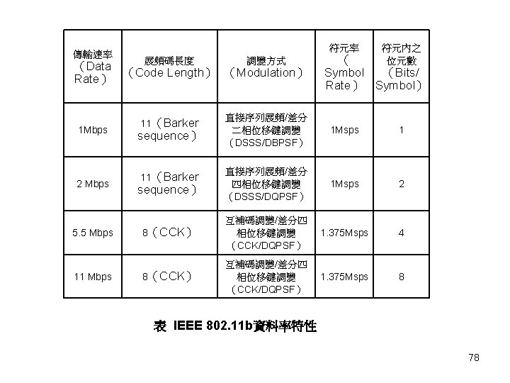
802. 11 Physical Layer • (1999) 802. 11 b (HR/DSSS at 2. 4 GHz) – 5. 5 Mbps and 11 Mbps • (1999) 802. 11 a (OFDM at 5 GHz) – 6 Mbps to 54 Mbps • (2003) 802. 11 g (OFDM at 2. 4 GHz) – Maximal rate: 54 Mbps – Maximal rate: get up to 108 Mbps (Atheros’ Super G) 74

802. 11 b • 802. 11 b - Data Transmission – Transmit 300 to 500 feet – Frequency-hopping spread-spectrum (FHSS) • 1 or 2 Mbps – Direct-sequence spread-spectrum (DSSS) • 1, 2, 5. 5, or 11 Mbps • 802. 11 b - Frequencies and Bandwidth – 2. 4000 to 2. 4835 GHz frequency – 22 MHz bandwidth per channel – 3 MHz guard bands 75

• Transmission – 1 and 2 Mbps speeds • Use 11 -bit Barker sequence • A Barker sequence is a string of digits of length such that for all – Higher data rate, 5. 5 and 11 Mbps speeds • Use complementary code keying (CCK) • The CCK is a variation and improvement on M-ary Orthogonal Keying Modulation. 76

CCK • CCK is a “single carrier” system, meaning that all data is transmitted by modulating a single radio frequency or carrier. Signal bandwidth Single carrier frequency 77

79

802. 11 a • 802. 11 a - Data Transmission – Transmit 100 to 150 feet – Orthogonal Frequency-Division Multiplexing (OFDM) • 6 to 54 Mbps • OFDM is a “multi-carrier” modulation scheme. • Data is split up among several closely spaced “subcarriers”, increasing reliability and speed • 802. 11 a - Frequencies and Bandwidth – 12 channels – 20 MHz bandwidth per channel – Broken into 52 separate channels 80 • 48 transmit, 4 used for control

Orthogonal Frequency Division Multiplexing – was first implemented in 802. 11 a. – OFDM is a “multi-carrier” modulation scheme. – Data is split up among several closely spaced “subcarriers” or frequencies, increasing reliability and speed 81

• Transmission – 6 and 9 Mbps speeds • Use 24 -bit Barker sequence • Lowest rate: 6 Mbps – BPSK - 48 bits per symbol, Rate 1/2 coding » 24 data bits per symbol » 24 x 250 ksps = 6 Mbps – 12, 24 and 28 Mbps speeds • Use binary phase shift keying (BPSK) 82

83

Comparison • Physical Layer 802. 11 b DSSS • 3 - 22 MHz channels • Data Rates: up to 11 Mbps (5. 5 is norm) • Frequency Range up to 300 Feet 802. 11 a OFDM • 12 – 20 MHz channels • Data rates: up to 54 Mbps (12 -24 is norm) • Frequency Range up to 300 Feet 84

Range Comparison 85

802. 11 g (Atheros’ Super G) How does Atheros’ Super G make 802. 11 g faster? 1. Compression – Link-level hardware compression utilizes the connection more efficiently and maximizes bandwidth. – In hardware compression, the compression computations are offloaded to a secondary hardware module. This frees the central CPU from the computationally intensive task of compression calculations. 86

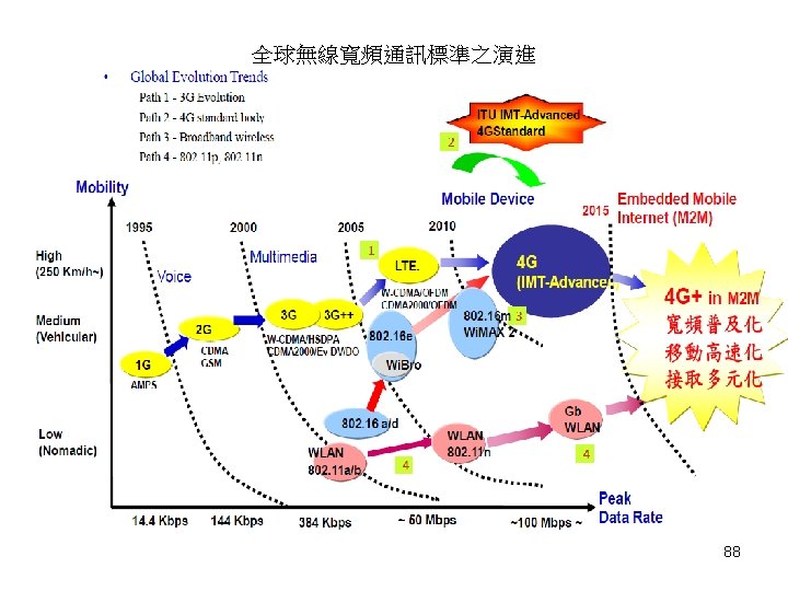
Push Toward High Data-Rate Systems Why Congested ? Multiple Antenna Systems Data rate 1 Gbps LTE (8 x 8 MIMO) 300 Mbps 802. 11 n (4 x 4 MIMO) Wi. Max (8 x 8 MIMO) 56 -128 Mbps 11 -54 Mbps 802. 11 a/b/g 56 -114 kbps 30 -40 kbps GPRS GSM 199 X 2000 87 Far below theoretical bound 2003 2009 2007 2012 year

IV. Wi. MAX • Wi. MAX Network Architecture • Recent Technologies in Wi. MAX – 802. 16 j – 802. 16 m • Overview of IEEE 802. 16 m • Advanced Features & Challenges of IEEE 802. 16 m 89

Wi. Max • Wi. MAX Forum – Wi. MAX: Worldwide Interoperability for Microwave Access – Formed in Apr 2001, by Intel, Proxim, Airspan, Fujitsu, etc. – 500+ members including Intel, R&S, Alvarion, Wavesat, Pico. Chip, Sony, Samsung, Nokia, TI, ADI, III, ITRI, etc. – Support IEEE 802. 16 standards • IEEE 802. 16 Standards – 802. 16 d/e define data and control plane functions in wireless PHY/MAC – 802. 16 f/g/i define management plane functions 90

Wi. MAX Network Architecture Inter-ASN Mobility: R 3, R 4 Intra-ASN Mobility: R 6, R 8 R 3 ASN GW R 4 R 6 R 6 R 8 Wi. MAX BS R 1 MS: Mobile Station Wi. MAX MS SS: Stationary Station Rx: Reference point x ASN GW: Access Service Network Gateway R 6 R 1 Wi. MAX MS R 1 Wi. MAX BS Wi. MAX SS 91

Recent Technologies in Wi. MAX • 802. 16 j Multi-hop Relay – Aiming at developing relay based on IEEE 802. 16 e, to gain: • Coverage extension • Throughput enhancement – Scope • To specify OFDMA PHY and MAC enhancement to IEEE Std. 802. 16 for licensed bands to enable the operation of relay stations • Subscriber station specifications are not changed • 802. 16 m – Advanced Air Interface for BWA in the future • Moving towards 4 G – Scope: • To amend the IEEE 802. 16 Wireless. MAN-OFDMA to provide an advanced air interface for operation in licensed bands • To meet the cellular layer requirements of IMT-Advanced next generation mobile networks • To provide continuing support for legacy Wireless. MAN-OFDMA equipment 92

Overview of IEEE 802. 16 m • IEEE 802. 16 m provides the performance improvements necessary to support future advanced services and applications for 4 G communications. • Major worldwide governmental and industrial organizations, including ARIB, TTA, and the Wi. MAX Forum, are adopting this standard. • IEEE 802. 16 m Support – – low to high mobility applications a wide range of data rates in multiple user environments high-quality multimedia applications significant improvements in performance and quality of service 93

MIMO architecture for the downlink of 802. 16 m systems. 94

Features of 802. 16 m • Aggregate Data Rate: – 100 Mbps for mobile stations, – 1 Gbps for fixed • Operating Radio Frequency: < 6 GHz • MIMO support: 4 or 8 streams, no limit on antennas • Coverage: 3 km, 5 -30 km and 30 -100 km 95

Advanced Features & Challenges of 16 m 1. Unified single-user/multi-user MIMO Architecture – support various advanced multi-antenna processing techniques including open-loop and closed single-user/multi-user MIMO schemes (single stream and multi-stream) – Support multi-cell MIMO techniques 2. Multi-carrier support – The RF carriers may be of different bandwidths and can be noncontiguous or belong to different frequency bands – The channels may be of different duplexing modes, e. g. FDD, TDD – Support wider band (up to 100 MHz) by BW aggregation across contiguous or non-contiguous channels 96

3. Multi-hop relay-enabled architecture – Improve the SINR in the cell for coverage extension and throughput enhancement 4. Support of femto-cells and self-organization – Femto-cells are low power BS at homes achieving FMC – Self-configuration by allowing real plug and play installation of network nodes and cells – Self-optimization by allowing automated or autonomous optimization of network performance with respect to service availability, Qo. S, network efficiency and throughput 97

5. Enhanced multicast and broadcast service – Multi-carriers with dedicated broadcast only carriers – Single/multi-BS MBS 6. Multi-rate operation and handover – Support interworking with IEEE 802. 11, GSM/EDGE, 3 GPP, 3 GPP 2, CDMA 2000 etc. 7. Multi-radio coexistence – MS reports its co-located radio activities to BS – Accordingly, BS can operates properly via scheduling to support multi-radio coexistence 98

References 1. 2. 3. 4. 5. 6. 7. 8. 9. Wi. MAX無線寬頻技術與垂直 智慧網通系統研究所 財團法人資訊 業策進會 Digital Signal Processing (4 th Edition): John G. Proakis Ioannis Papapanagiotou, Dimitris Toumpakaris, Jungwon Lee, Michael Devetsikiotis, “A Survey of Mobile Wi. MAX IEEE 802. 16 m Standard” IEEE COMMUNICATIONS SURVEYS & TUTORIALS, VOL. 11, NO. 4, FOURTH QUARTER 2009 IEEE 802. 11: Wireless LAN Medium Access Control (MAC) and Physical Layer (PHY) Specifications "802. 11 a-1999 High-speed Physical Layer in the 5 GHz band“ "802. 11 b-1999 Higher Speed Physical Layer Extension in the 2. 4 GHz band“ "IEEE 802. 11 g-2003: Further Higher Data Rate Extension in the 2. 4 GHz Band“ http: //zh. wikipedia. org/wiki/IEEE_802. 11 Shu Lin, Daniel J. Costello, (1983). “Error Control Coding: Fundamentals and Applications”

10. Shannon, C. E. (1948), "A Mathematical Theory of Communication", Bell System Technical Journal, 27, pp. 379– 423 & 623– 656, July & October, 1948. 11. John G. Proakis, Dimitris Manolakis: Digital Signal Processing - Principles, Algorithms and Applications 12. Lung-Sheng Tsai, Wei-Ho Chung*, and Da-Shan Shiu, "Lower Bounds on the Correlation Property for OFDM Sequences with Spectral-Null Constraints, " IEEE Transactions on Wireless Communications, Volume 10, Issue 8, pp. 2652 -2659, August 2011. 13. Lung-Sheng Tsai, Wei-Ho Chung*, and Da-Shan Shiu, "Synthesizing Low Autocorrelation and Low PAPR OFDM Sequences Under Spectral Constraints Through Convex Optimization and GS Algorithm, " IEEE Transactions on Signal Processing, Volume 59, Issue 5, pp. 2234 -2243, May 2011. 14. Ronald Y. Chang, Sian-Jheng Lin, and Wei-Ho Chung, "Efficient Implementation of the MIMO Sphere Detector: Architecture and Complexity Analysis, " IEEE Transactions on Vehicular Technology, 2012 15. Ronald Y. Chang and Wei-Ho Chung*, "Best-First Tree Search with Probabilistic Node Ordering for MIMO Detection: Generalization and Performance-Complexity Tradeoff, " IEEE Transactions on Wireless 100 Communications, 2012.

Thank you whc@citi. sinica. edu. tw 101