ESTIMATING THE STATE OF LARGE SPATIOTEMPORALLY CHAOTIC SYSTEMS

ESTIMATING THE STATE OF LARGE SPATIOTEMPORALLY CHAOTIC SYSTEMS: WEATHER FORECASTING, ETC. Edward Ott University of Maryland Main Reference: E. OTT, B. HUNT, I. SZUNYOGH, A. V. ZIMIN, E. KOSTELICH, M. CORAZZA, E. KALNAY, D. J. PATIL, & J. YORKE, TELLUS A (2004). http: //www. weatherchaos. umd. edu/ 1

OUTLINE • Review of some basic aspects of weather forecasting. • Our method in brief. • Tests of our method. 2

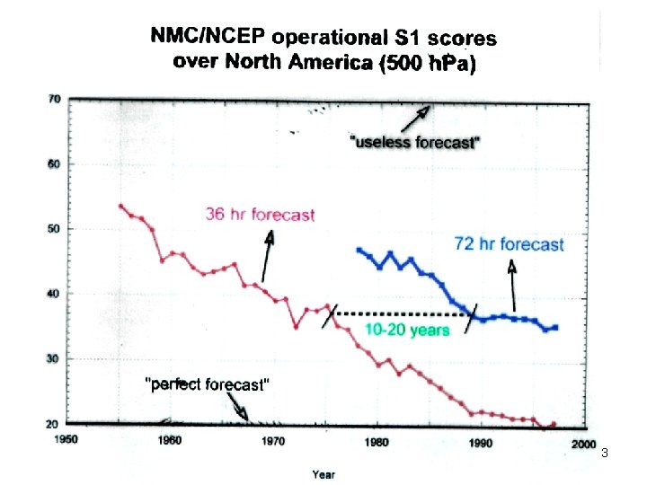
3

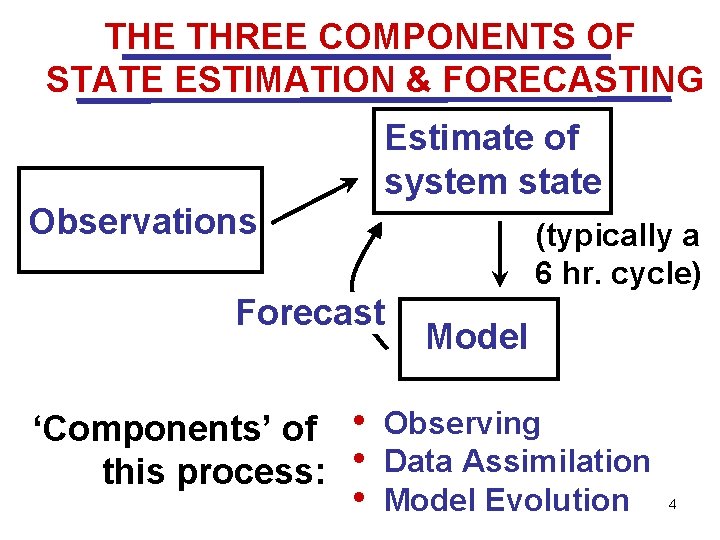
THE THREE COMPONENTS OF STATE ESTIMATION & FORECASTING Estimate of system state Observations (typically a 6 hr. cycle) Forecast Model ‘Components’ of • Observing this process: • Data Assimilation • Model Evolution 4

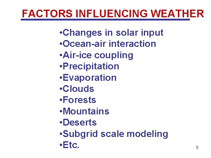
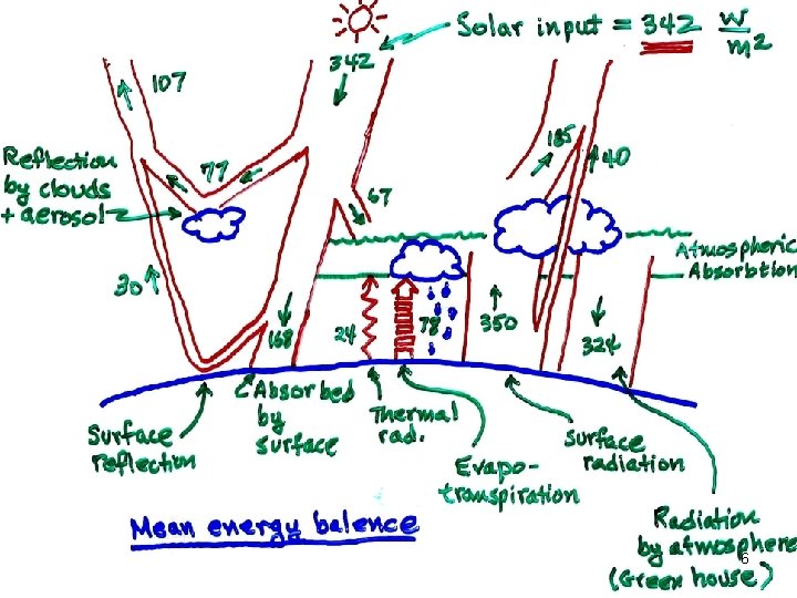
FACTORS INFLUENCING WEATHER • Changes in solar input • Ocean-air interaction • Air-ice coupling • Precipitation • Evaporation • Clouds • Forests • Mountains • Deserts • Subgrid scale modeling • Etc. 5

6

7

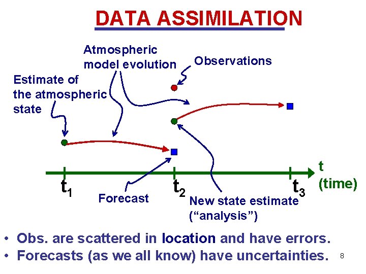
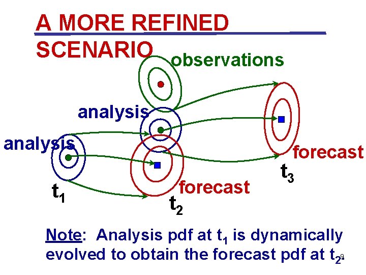
DATA ASSIMILATION Atmospheric model evolution Observations Estimate of the atmospheric state t 1 Forecast t 2 t 3 t (time) New state estimate (“analysis”) • Obs. are scattered in location and have errors. • Forecasts (as we all know) have uncertainties. 8

A MORE REFINED SCENARIO observations analysis t 1 forecast t 3 t 2 Note: Analysis pdf at t 1 is dynamically evolved to obtain the forecast pdf at t 29.

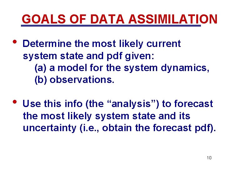
GOALS OF DATA ASSIMILATION • Determine the most likely current system state and pdf given: (a) a model for the system dynamics, (b) observations. • Use this info (the “analysis”) to forecast the most likely system state and its uncertainty (i. e. , obtain the forecast pdf). 10

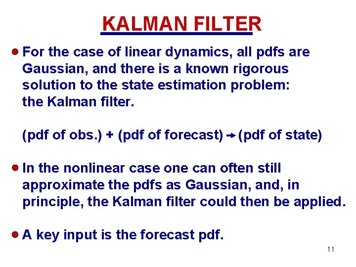
KALMAN FILTER For the case of linear dynamics, all pdfs are Gaussian, and there is a known rigorous solution to the state estimation problem: the Kalman filter. (pdf of obs. ) + (pdf of forecast) (pdf of state) In the nonlinear case one can often still approximate the pdfs as Gaussian, and, in principle, the Kalman filter could then be applied. A key input is the forecast pdf. 11

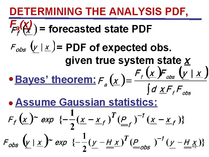
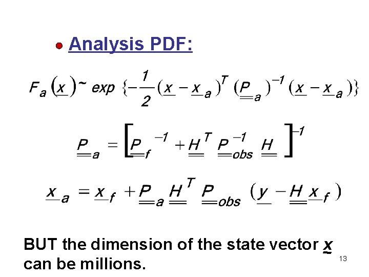
DETERMINING THE ANALYSIS PDF, Fa(x) = forecasted state PDF = PDF of expected obs. given true system state x Bayes’ theorem: Assume Gaussian statistics: 12

Analysis PDF: BUT the dimension of the state vector x can be millions. 13

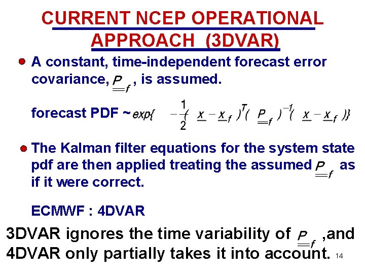
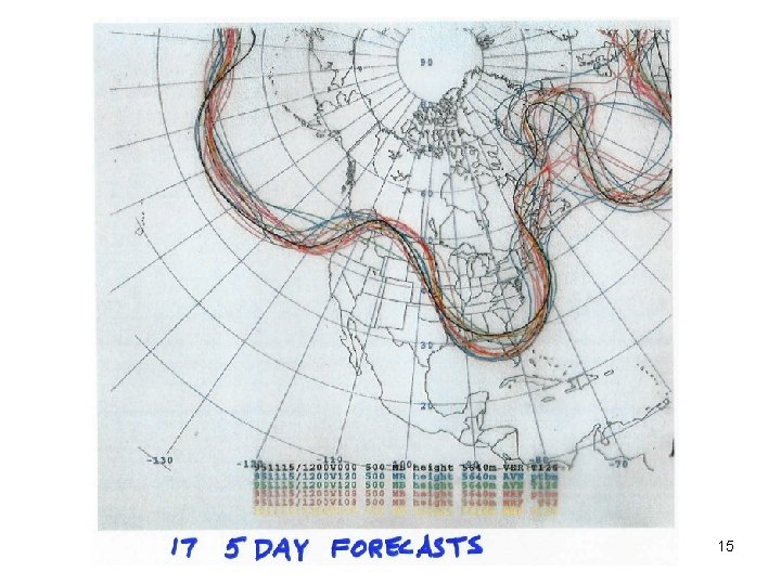
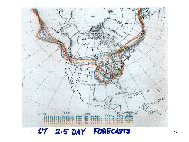
CURRENT NCEP OPERATIONAL APPROACH (3 DVAR) A constant, time-independent forecast error covariance, , is assumed. forecast PDF ~ The Kalman filter equations for the system state pdf are then applied treating the assumed as if it were correct. ECMWF : 4 DVAR 3 DVAR ignores the time variability of , and 4 DVAR only partially takes it into account. 14

15

16

PROBLEM Currently data assimilation is already a very computationally costly part of operational numerical weather prediction. Implementation of a full Kalman filter would be many times more costly, and is impractical for the foreseeable future. 17

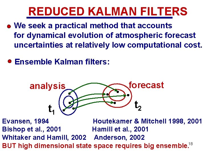
REDUCED KALMAN FILTERS We seek a practical method that accounts for dynamical evolution of atmospheric forecast uncertainties at relatively low computational cost. Ensemble Kalman filters: analysis t 1 forecast t 2 Evansen, 1994 Houtekamer & Mitchell 1998, 2001 Bishop et al. , 2001 Hamill et al. , 2001 Whitaker and Hamill, 2002 Anderson, 2002 BUT high dimensional state space requires big ensemble. 18

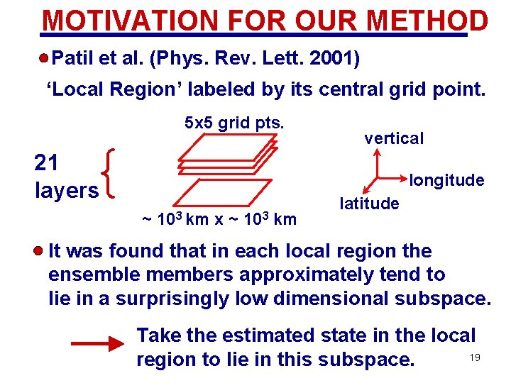
MOTIVATION FOR OUR METHOD Patil et al. (Phys. Rev. Lett. 2001) ‘Local Region’ labeled by its central grid point. 5 x 5 grid pts. { 21 layers vertical longitude ~ 103 km x ~ 103 km latitude It was found that in each local region the ensemble members approximately tend to lie in a surprisingly low dimensional subspace. Take the estimated state in the local 19 region to lie in this subspace.

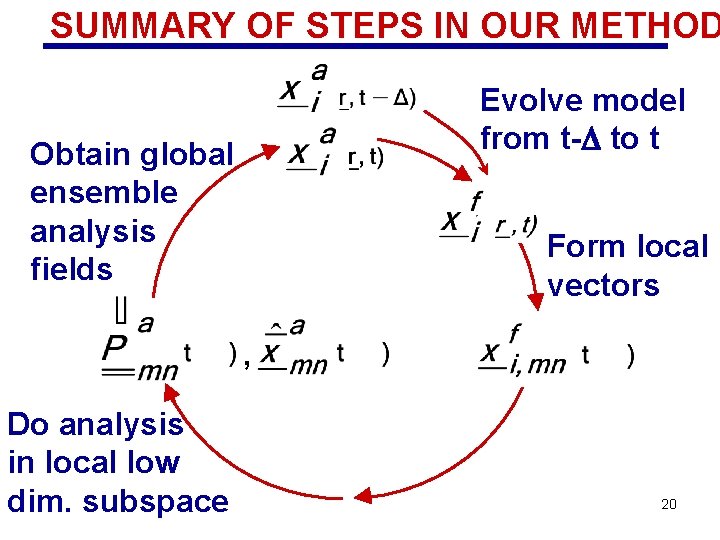
SUMMARY OF STEPS IN OUR METHOD Evolve model from t-D to t Obtain global ensemble analysis fields Form local vectors , Do analysis in local low dim. subspace 20

PROPERTIES OF OUR METHOD Only operations on relatively small matrices are needed in the analyses. (We work in the local low dimensional subspaces. ) The analyses in each local region are independent. Fast parallel computations are possible. 21

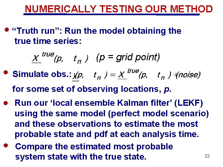
NUMERICALLY TESTING OUR METHOD “Truth run”: Run the model obtaining the true time series: (p = grid point) Simulate obs. : for some set of observing locations, p. Run our ‘local ensemble Kalman filter’ (LEKF) using the same model (perfect model scenario) and these observations to estimate the most probable state and pdf at each analysis time. Compare the estimated most probable 22 system state with the true state.

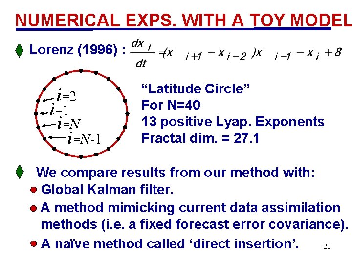
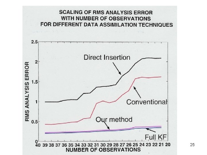
NUMERICAL EXPS. WITH A TOY MODEL Lorenz (1996) : i =2 i =1 i =N i=N-1 “Latitude Circle” For N=40 13 positive Lyap. Exponents Fractal dim. = 27. 1 We compare results from our method with: Global Kalman filter. A method mimicking current data assimilation methods (i. e. a fixed forecast error covariance). A naïve method called ‘direct insertion’. 23

24

25

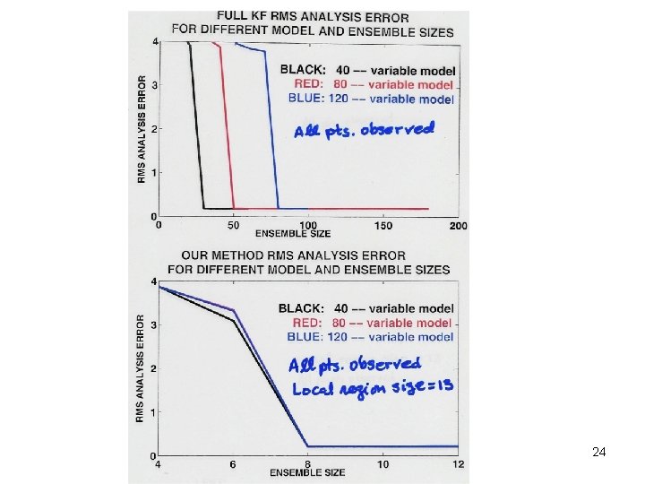
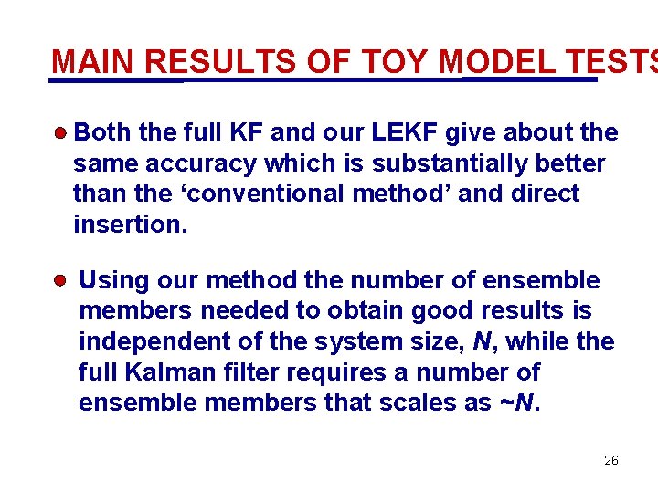
MAIN RESULTS OF TOY MODEL TESTS Both the full KF and our LEKF give about the same accuracy which is substantially better than the ‘conventional method’ and direct insertion. Using our method the number of ensemble members needed to obtain good results is independent of the system size, N, while the full Kalman filter requires a number of ensemble members that scales as ~N. 26

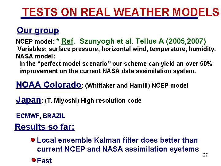
TESTS ON REAL WEATHER MODELS Our group NCEP model: * Ref. Szunyogh et al. Tellus A (2005, 2007) Variables: surface pressure, horizontal wind, temperature, humidity. NASA model: In the “perfect model scenario” our scheme can yield an over 50% improvement on the current NASA data assimilation system. NOAA Colorado: (Whittaker and Hamill) NCEP model Japan: (T. Miyoshi) High resolution code ECMWF, BRAZIL Results so far: Local ensemble Kalman filter does better than current NCEP and NASA assimilation systems Fast 27

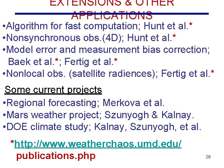
EXTENSIONS & OTHER APPLICATIONS • Algorithm for fast computation; Hunt et al. * • Nonsynchronous obs. (4 D); Hunt et al. * • Model error and measurement bias correction; Baek et al. *; Fertig et al. * • Nonlocal obs. (satellite radiences); Fertig et al. * Some current projects • Regional forecasting; Merkova et al. • Mars weather project; Szunyogh & Kalnay. • DOE climate study; Kalnay, Szunyogh, et al. *http: //www. weatherchaos. umd. edu/ publications. php 28

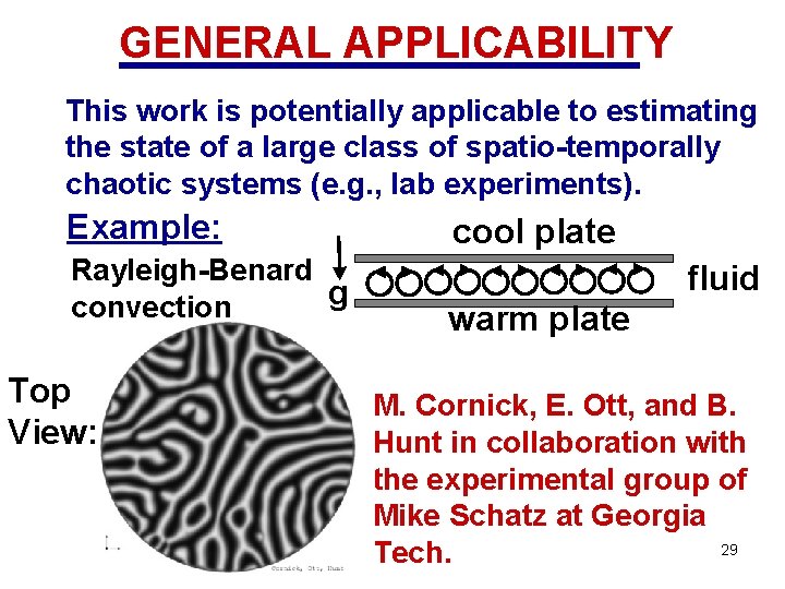
GENERAL APPLICABILITY This work is potentially applicable to estimating the state of a large class of spatio-temporally chaotic systems (e. g. , lab experiments). Example: Rayleigh-Benard g convection Top View: cool plate fluid warm plate M. Cornick, E. Ott, and B. Hunt in collaboration with the experimental group of Mike Schatz at Georgia 29 Tech.

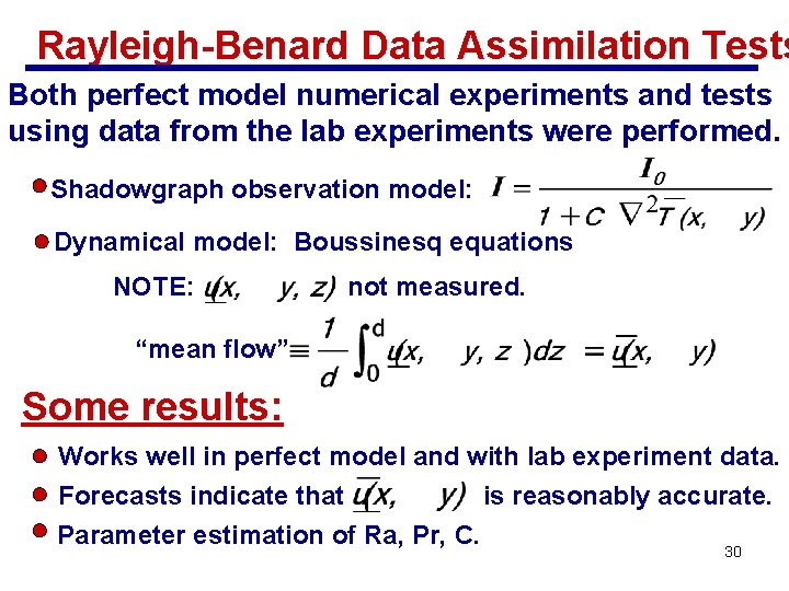
Rayleigh-Benard Data Assimilation Tests Both perfect model numerical experiments and tests using data from the lab experiments were performed. Shadowgraph observation model: Dynamical model: Boussinesq equations NOTE: not measured. “mean flow” Some results: Works well in perfect model and with lab experiment data. Forecasts indicate that is reasonably accurate. Parameter estimation of Ra, Pr, C. 30

PROPERTIES OF THE METHOD Only low dimensional matrix operations are used in the analysis. Local analyses are independent and hence parallelizable. Potentially fast and accurate. http: //www. weatherchaos. umd. edu/ publications. php 31

32

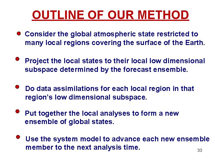
OUTLINE OF OUR METHOD Consider the global atmospheric state restricted to many local regions covering the surface of the Earth. Project the local states to their local low dimensional subspace determined by the forecast ensemble. Do data assimilations for each local region in that region’s low dimensional subspace. Put together the local analyses to form a new ensemble of global states. Use the system model to advance each new ensemble member to the next analysis time. 33