Estimating with Confidence Estimating with Confidence n Confidence

+ Estimating with Confidence

+ Estimating with Confidence n Confidence Intervals: The Basics n Estimating a Population Proportion n Estimating a Population Mean

+ Confidence Intervals: The Basics Learning Objectives After this section, you should be able to… ü INTERPRET a confidence level ü INTERPRET a confidence interval in context ü DESCRIBE how a confidence interval gives a range of plausible values for the parameter ü DESCRIBE the inference conditions necessary to construct confidence intervals ü EXPLAIN practical issues that can affect the interpretation of a confidence interval

We learned that different samples yield different results for our estimate. Statistical inference uses the language of probability to express the strength of our conclusions by taking chance variation due to random selection or random assignment into account. In this section, we’ll learn one method of statistical inference – confidence intervals – so we may estimate the value of a parameter from a sample statistic. As we do so, we’ll learn not only how to construct a confidence interval, but also how to report probabilities that would describe what would happen if we used the inference method many times. Confidence Intervals: The Basics Our goal in many statistical settings is to use a sample statistic to estimate a population parameter. In Chapter 4, we learned if we randomly select the sample, we should be able to generalize our results to the population of interest. + n Introduction

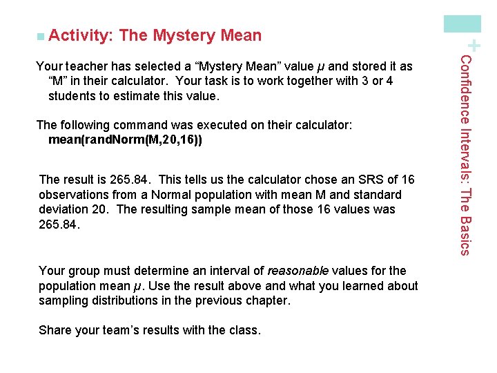
The Mystery Mean The following command was executed on their calculator: mean(rand. Norm(M, 20, 16)) The result is 265. 84. This tells us the calculator chose an SRS of 16 observations from a Normal population with mean M and standard deviation 20. The resulting sample mean of those 16 values was 265. 84. Your group must determine an interval of reasonable values for the population mean µ. Use the result above and what you learned about sampling distributions in the previous chapter. Share your team’s results with the class. Confidence Intervals: The Basics Your teacher has selected a “Mystery Mean” value µ and stored it as “M” in their calculator. Your task is to work together with 3 or 4 students to estimate this value. + n Activity:

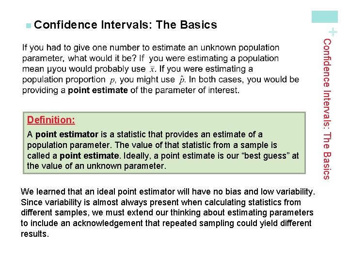
Intervals: The Basics A point estimator is a statistic that provides an estimate of a population parameter. The value of that statistic from a sample is called a point estimate. Ideally, a point estimate is our “best guess” at the value of an unknown parameter. We learned that an ideal point estimator will have no bias and low variability. Since variability is almost always present when calculating statistics from different samples, we must extend our thinking about estimating parameters to include an acknowledgement that repeated sampling could yield different results. Confidence Intervals: The Basics Definition: + n Confidence

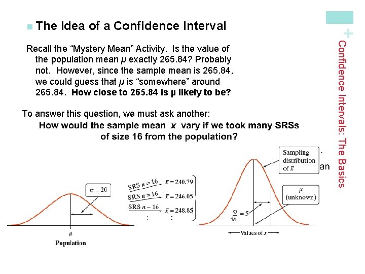
Idea of a Confidence Interval To answer this question, we must ask another: Confidence Intervals: The Basics Recall the “Mystery Mean” Activity. Is the value of the population mean µ exactly 265. 84? Probably not. However, since the sample mean is 265. 84, we could guess that µ is “somewhere” around 265. 84. How close to 265. 84 is µ likely to be? + n The

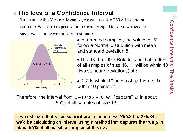
Idea of a Confidence Interval + n The Confidence Intervals: The Basics If we estimate that µ lies somewhere in the interval 255. 84 to 275. 84, we’d be calculating an interval using a method that captures the true µ in about 95% of all possible samples of this size.

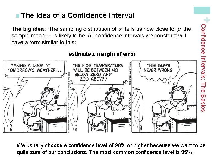
Idea of a Confidence Interval Definition: A confidence interval for a parameter has two parts: • An interval calculated from the data, which has the form: estimate ± margin of error • The margin of error tells how close the estimate tends to be to the unknown parameter in repeated random sampling. • A confidence level C, the overall success rate of the method for calculating the confidence interval. That is, in C% of all possible samples, the method would yield an interval that captures the true parameter value. Confidence Intervals: The Basics estimate ± margin of error + n The We usually choose a confidence level of 90% or higher because we want to be quite sure of our conclusions. The most common confidence level is 95%.

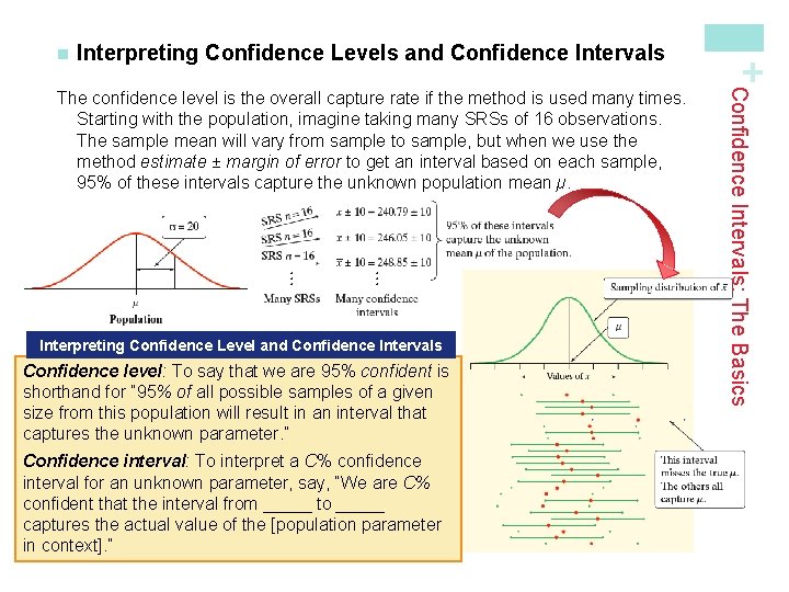
Interpreting Confidence Levels and Confidence Intervals Interpreting Confidence Level and Confidence Intervals Confidence level: To say that we are 95% confident is shorthand for “ 95% of all possible samples of a given size from this population will result in an interval that captures the unknown parameter. ” Confidence interval: To interpret a C% confidence interval for an unknown parameter, say, “We are C% confident that the interval from _____ to _____ captures the actual value of the [population parameter in context]. ” Confidence Intervals: The Basics The confidence level is the overall capture rate if the method is used many times. Starting with the population, imagine taking many SRSs of 16 observations. The sample mean will vary from sample to sample, but when we use the method estimate ± margin of error to get an interval based on each sample, 95% of these intervals capture the unknown population mean µ. + n

Interpreting Confidence Levels and Confidence Intervals The confidence level does not tell us the chance that a particular confidence interval captures the population parameter. Instead, the confidence interval gives us a set of plausible values for the parameter. We interpret confidence levels and confidence intervals in much the same way whether we are estimating a population mean, proportion, or some other parameter. Confidence Intervals: The Basics The confidence level tells us how likely it is that the method we are using will produce an interval that captures the population parameter if we use it many times. + n

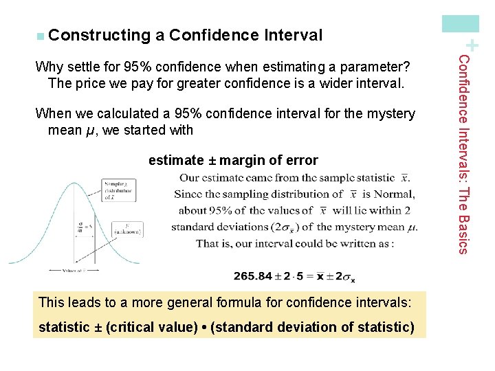
a Confidence Interval When we calculated a 95% confidence interval for the mystery mean µ, we started with estimate ± margin of error This leads to a more general formula for confidence intervals: statistic ± (critical value) • (standard deviation of statistic) Confidence Intervals: The Basics Why settle for 95% confidence when estimating a parameter? The price we pay for greater confidence is a wider interval. + n Constructing

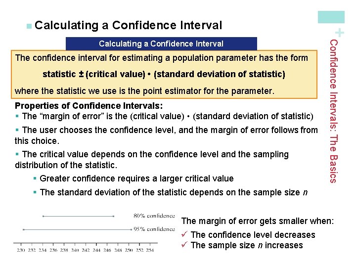
a Confidence Interval The confidence interval for estimating a population parameter has the form statistic ± (critical value) • (standard deviation of statistic) where the statistic we use is the point estimator for the parameter. Properties of Confidence Intervals: § The “margin of error” is the (critical value) • (standard deviation of statistic) § The user chooses the confidence level, and the margin of error follows from this choice. § The critical value depends on the confidence level and the sampling distribution of the statistic. § Greater confidence requires a larger critical value § The standard deviation of the statistic depends on the sample size n Confidence Intervals: The Basics Calculating a Confidence Interval + n Calculating The margin of error gets smaller when: ü The confidence level decreases ü The sample size n increases

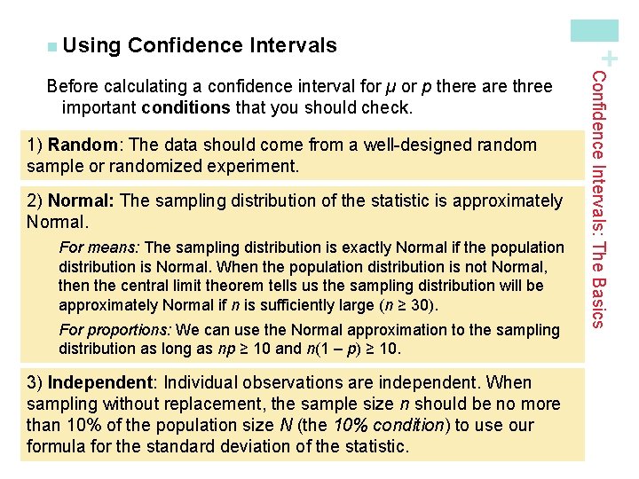
Confidence Intervals 1) Random: The data should come from a well-designed random sample or randomized experiment. 2) Normal: The sampling distribution of the statistic is approximately Normal. For means: The sampling distribution is exactly Normal if the population distribution is Normal. When the population distribution is not Normal, then the central limit theorem tells us the sampling distribution will be approximately Normal if n is sufficiently large (n ≥ 30). For proportions: We can use the Normal approximation to the sampling distribution as long as np ≥ 10 and n(1 – p) ≥ 10. 3) Independent: Individual observations are independent. When sampling without replacement, the sample size n should be no more than 10% of the population size N (the 10% condition) to use our formula for the standard deviation of the statistic. Confidence Intervals: The Basics Before calculating a confidence interval for µ or p there are three important conditions that you should check. + n Using

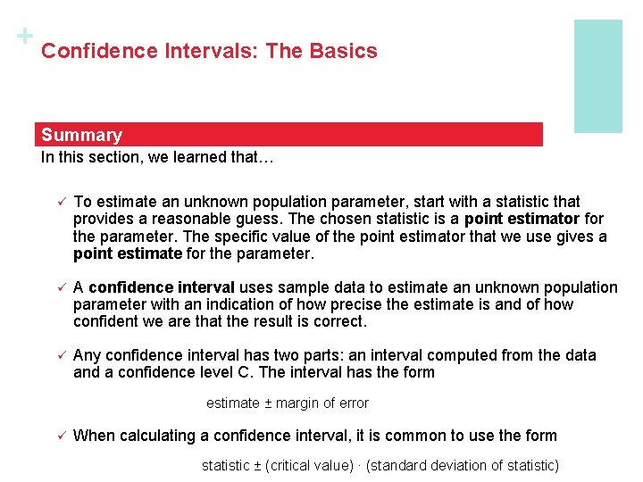
+ Confidence Intervals: The Basics Summary In this section, we learned that… ü To estimate an unknown population parameter, start with a statistic that provides a reasonable guess. The chosen statistic is a point estimator for the parameter. The specific value of the point estimator that we use gives a point estimate for the parameter. ü A confidence interval uses sample data to estimate an unknown population parameter with an indication of how precise the estimate is and of how confident we are that the result is correct. ü Any confidence interval has two parts: an interval computed from the data and a confidence level C. The interval has the form estimate ± margin of error ü When calculating a confidence interval, it is common to use the form statistic ± (critical value) · (standard deviation of statistic)

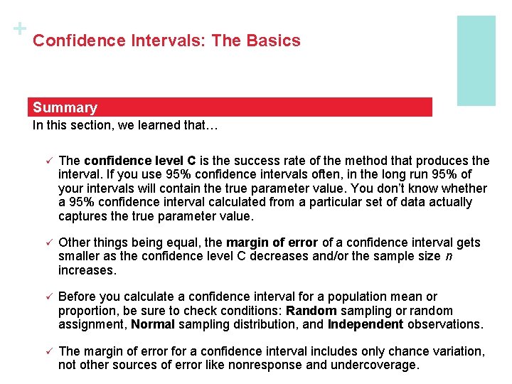
+ Confidence Intervals: The Basics Summary In this section, we learned that… ü The confidence level C is the success rate of the method that produces the interval. If you use 95% confidence intervals often, in the long run 95% of your intervals will contain the true parameter value. You don’t know whether a 95% confidence interval calculated from a particular set of data actually captures the true parameter value. ü Other things being equal, the margin of error of a confidence interval gets smaller as the confidence level C decreases and/or the sample size n increases. ü Before you calculate a confidence interval for a population mean or proportion, be sure to check conditions: Random sampling or random assignment, Normal sampling distribution, and Independent observations. ü The margin of error for a confidence interval includes only chance variation, not other sources of error like nonresponse and undercoverage.

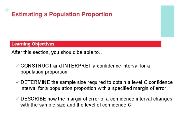
+ Estimating a Population Proportion Learning Objectives After this section, you should be able to… ü CONSTRUCT and INTERPRET a confidence interval for a population proportion ü DETERMINE the sample size required to obtain a level C confidence interval for a population proportion with a specified margin of error ü DESCRIBE how the margin of error of a confidence interval changes with the sample size and the level of confidence C

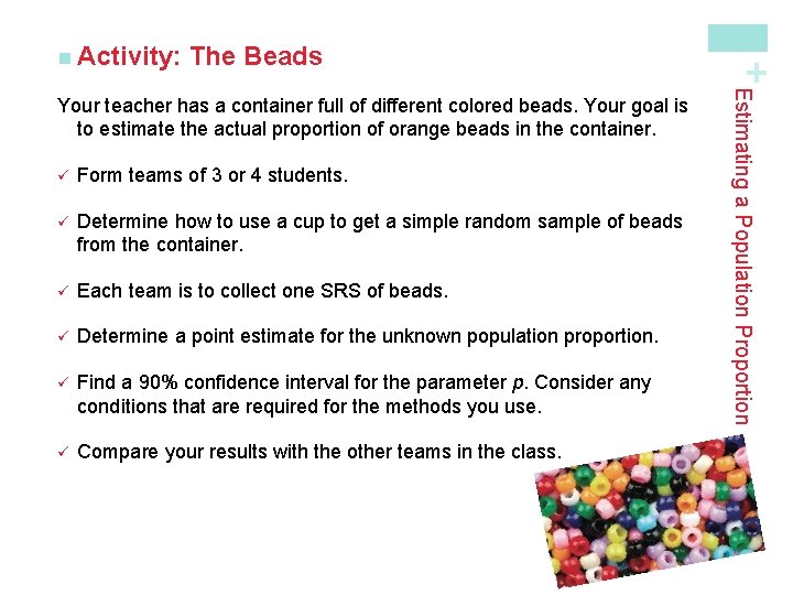
The Beads ü Form teams of 3 or 4 students. ü Determine how to use a cup to get a simple random sample of beads from the container. ü Each team is to collect one SRS of beads. ü Determine a point estimate for the unknown population proportion. ü Find a 90% confidence interval for the parameter p. Consider any conditions that are required for the methods you use. ü Compare your results with the other teams in the class. Estimating a Population Proportion Your teacher has a container full of different colored beads. Your goal is to estimate the actual proportion of orange beads in the container. + n Activity:

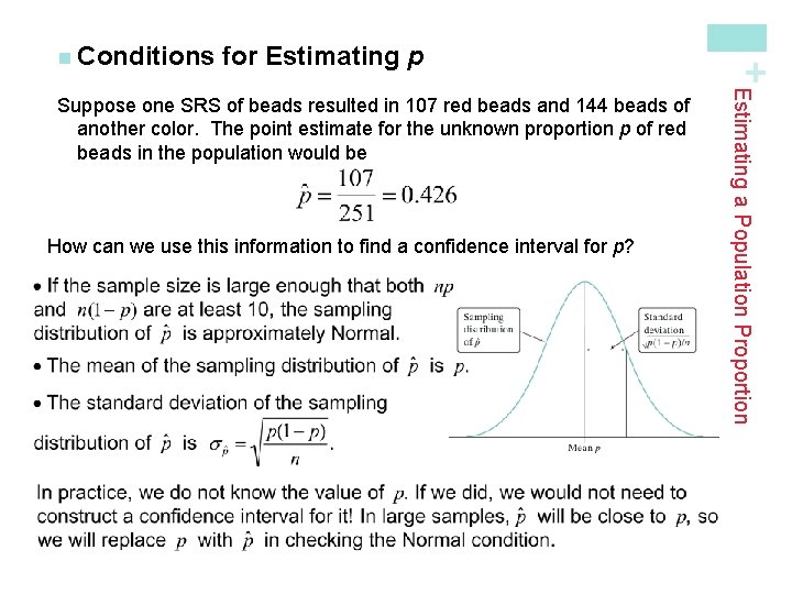
for Estimating p How can we use this information to find a confidence interval for p? Estimating a Population Proportion Suppose one SRS of beads resulted in 107 red beads and 144 beads of another color. The point estimate for the unknown proportion p of red beads in the population would be + n Conditions

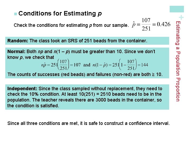
for Estimating p Random: The class took an SRS of 251 beads from the container. Normal: Both np and n(1 – p) must be greater than 10. Since we don’t know p, we check that The counts of successes (red beads) and failures (non-red) are both ≥ 10. Independent: Since the class sampled without replacement, they need to check the 10% condition. At least 10(251) = 2510 beads need to be in the population. The teacher reveals there are 3000 beads in the container, so the condition is satisfied. Since all three conditions are met, it is safe to construct a confidence interval. Estimating a Population Proportion Check the conditions for estimating p from our sample. + n Conditions

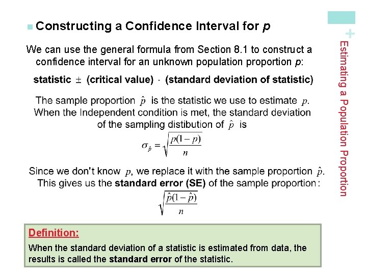
a Confidence Interval for p Definition: When the standard deviation of a statistic is estimated from data, the results is called the standard error of the statistic. Estimating a Population Proportion We can use the general formula from Section 8. 1 to construct a confidence interval for an unknown population proportion p: + n Constructing

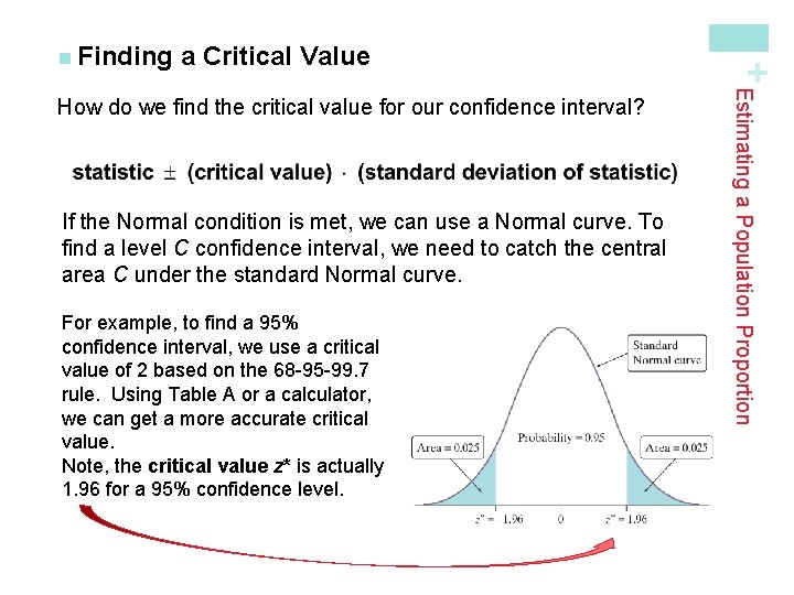
a Critical Value If the Normal condition is met, we can use a Normal curve. To find a level C confidence interval, we need to catch the central area C under the standard Normal curve. For example, to find a 95% confidence interval, we use a critical value of 2 based on the 68 -95 -99. 7 rule. Using Table A or a calculator, we can get a more accurate critical value. Note, the critical value z* is actually 1. 96 for a 95% confidence level. Estimating a Population Proportion How do we find the critical value for our confidence interval? + n Finding

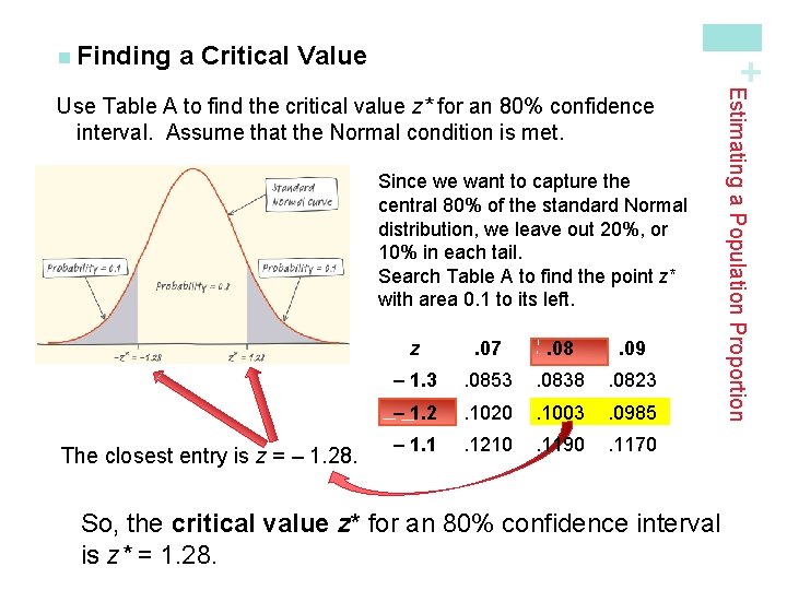
a Critical Value + n Finding Since we want to capture the central 80% of the standard Normal distribution, we leave out 20%, or 10% in each tail. Search Table A to find the point z* with area 0. 1 to its left. The closest entry is z = – 1. 28. z . 07 . 08 . 09 – 1. 3 . 0853 . 0838 . 0823 – 1. 2 . 1020 . 1003 . 0985 – 1. 1 . 1210 . 1190 . 1170 So, the critical value z* for an 80% confidence interval is z* = 1. 28. Estimating a Population Proportion Use Table A to find the critical value z* for an 80% confidence interval. Assume that the Normal condition is met.

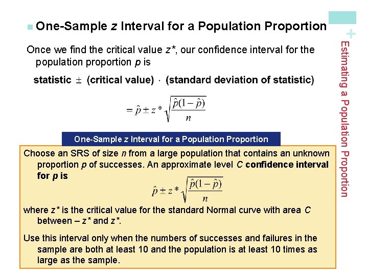
z Interval for a Population Proportion One-Sample z Interval for a Population Proportion Choose an SRS of size n from a large population that contains an unknown proportion p of successes. An approximate level C confidence interval for p is where z* is the critical value for the standard Normal curve with area C between – z* and z*. Use this interval only when the numbers of successes and failures in the sample are both at least 10 and the population is at least 10 times as large as the sample. Estimating a Population Proportion Once we find the critical value z*, our confidence interval for the population proportion p is + n One-Sample

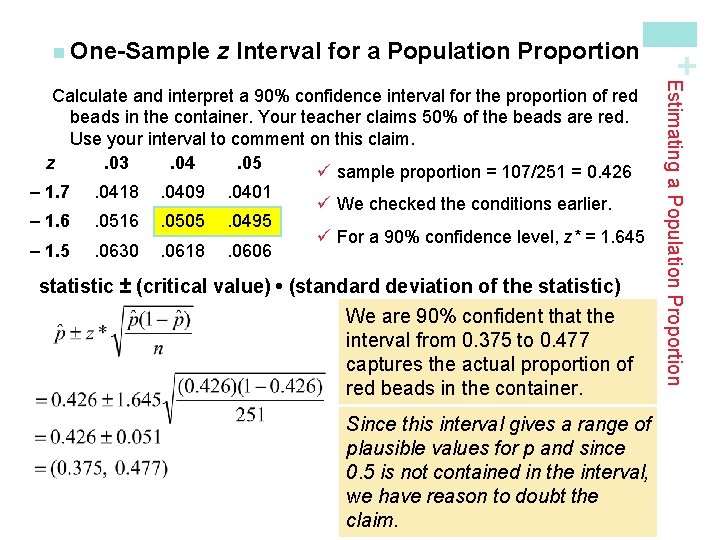
z Interval for a Population Proportion – 1. 7 . 0418 . 0409 . 0401 – 1. 6 . 0516 . 0505 . 0495 – 1. 5 . 0630 . 0618 . 0606 ü We checked the conditions earlier. ü For a 90% confidence level, z* = 1. 645 statistic ± (critical value) • (standard deviation of the statistic) We are 90% confident that the interval from 0. 375 to 0. 477 captures the actual proportion of red beads in the container. Since this interval gives a range of plausible values for p and since 0. 5 is not contained in the interval, we have reason to doubt the claim. Estimating a Population Proportion Calculate and interpret a 90% confidence interval for the proportion of red beads in the container. Your teacher claims 50% of the beads are red. Use your interval to comment on this claim. z. 03. 04. 05 ü sample proportion = 107/251 = 0. 426 + n One-Sample

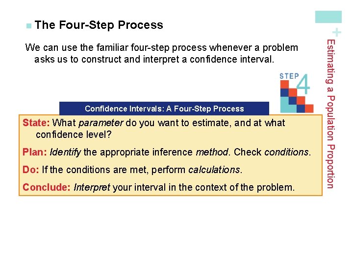
Four-Step Process Confidence Intervals: A Four-Step Process State: What parameter do you want to estimate, and at what confidence level? Plan: Identify the appropriate inference method. Check conditions. Do: If the conditions are met, perform calculations. Conclude: Interpret your interval in the context of the problem. Estimating a Population Proportion We can use the familiar four-step process whenever a problem asks us to construct and interpret a confidence interval. + n The

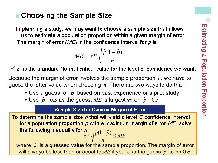
the Sample Size ü z* is the standard Normal critical value for the level of confidence we want. Sample Size for Desired Margin of Error To determine the sample size n that will yield a level C confidence interval for a population proportion p with a maximum margin of error ME, solve the following inequality for n: Estimating a Population Proportion In planning a study, we may want to choose a sample size that allows us to estimate a population proportion within a given margin of error. The margin of error (ME) in the confidence interval for p is + n Choosing

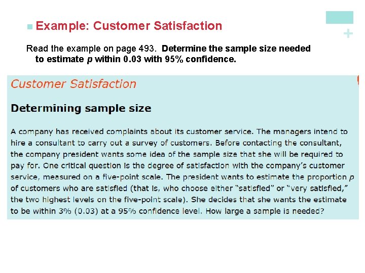
Customer Satisfaction Read the example on page 493. Determine the sample size needed to estimate p within 0. 03 with 95% confidence. + n Example:

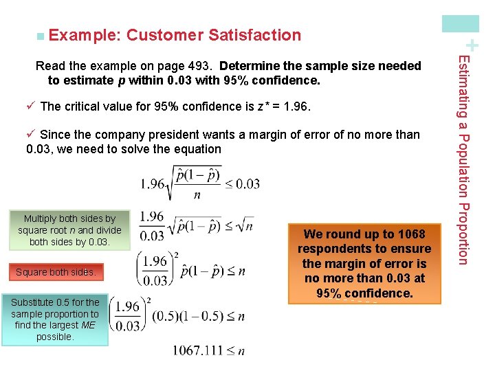
Customer Satisfaction ü The critical value for 95% confidence is z* = 1. 96. ü Since the company president wants a margin of error of no more than 0. 03, we need to solve the equation Multiply both sides by square root n and divide both sides by 0. 03. Square both sides. Substitute 0. 5 for the sample proportion to find the largest ME possible. We round up to 1068 respondents to ensure the margin of error is no more than 0. 03 at 95% confidence. Estimating a Population Proportion Read the example on page 493. Determine the sample size needed to estimate p within 0. 03 with 95% confidence. + n Example:

+ Estimating a Population Mean Learning Objectives After this section, you should be able to… ü CONSTRUCT and INTERPRET a confidence interval for a population mean ü DETERMINE the sample size required to obtain a level C confidence interval for a population mean with a specified margin of error ü DESCRIBE how the margin of error of a confidence interval changes with the sample size and the level of confidence C ü DETERMINE sample statistics from a confidence interval

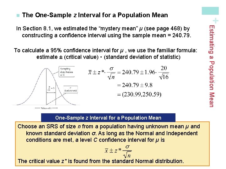
The One-Sample z Interval for a Population Mean To calculate a 95% confidence interval for µ , we use the familiar formula: estimate ± (critical value) • (standard deviation of statistic) One-Sample z Interval for a Population Mean Choose an SRS of size n from a population having unknown mean µ and known standard deviation σ. As long as the Normal and Independent conditions are met, a level C confidence interval for µ is The critical value z* is found from the standard Normal distribution. Estimating a Population Mean In Section 8. 1, we estimated the “mystery mean” µ (see page 468) by constructing a confidence interval using the sample mean = 240. 79. + n

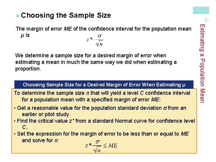
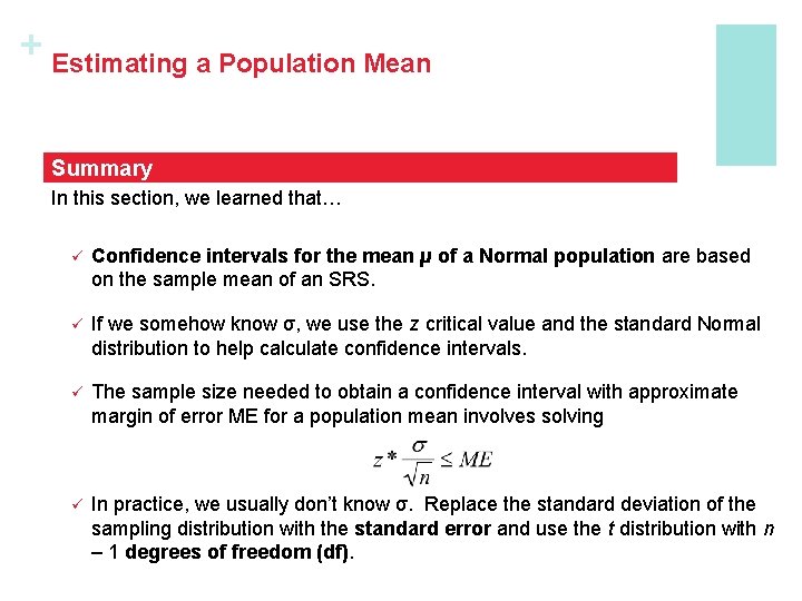
the Sample Size We determine a sample size for a desired margin of error when estimating a mean in much the same way we did when estimating a proportion. Choosing Sample Size for a Desired Margin of Error When Estimating µ To determine the sample size n that will yield a level C confidence interval for a population mean with a specified margin of error ME: • Get a reasonable value for the population standard deviation σ from an earlier or pilot study. • Find the critical value z* from a standard Normal curve for confidence level C. • Set the expression for the margin of error to be less than or equal to ME and solve for n: Estimating a Population Mean The margin of error ME of the confidence interval for the population mean µ is + n Choosing

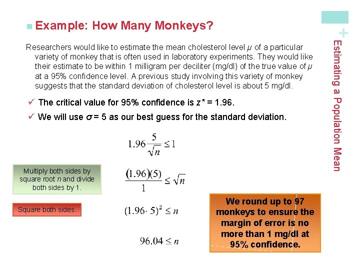
How Many Monkeys? + n Example: ü The critical value for 95% confidence is z* = 1. 96. ü We will use σ = 5 as our best guess for the standard deviation. Multiply both sides by square root n and divide both sides by 1. Square both sides. We round up to 97 monkeys to ensure the margin of error is no more than 1 mg/dl at 95% confidence. Estimating a Population Mean Researchers would like to estimate the mean cholesterol level µ of a particular variety of monkey that is often used in laboratory experiments. They would like their estimate to be within 1 milligram per deciliter (mg/dl) of the true value of µ at a 95% confidence level. A previous study involving this variety of monkey suggests that the standard deviation of cholesterol level is about 5 mg/dl.

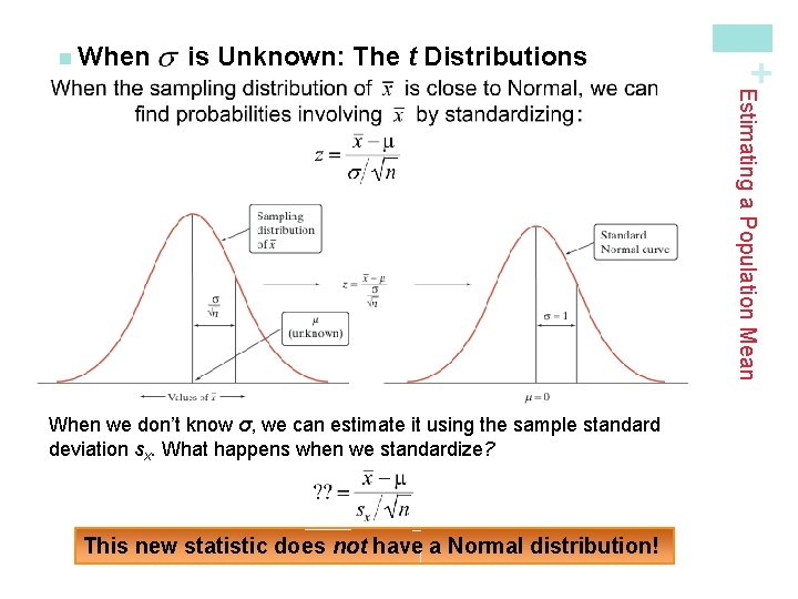
is Unknown: The t Distributions + n When Estimating a Population Mean When we don’t know σ, we can estimate it using the sample standard deviation sx. What happens when we standardize? This new statistic does not have a Normal distribution!

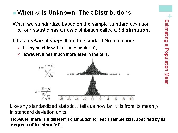
is Unknown: The t Distributions It has a different shape than the standard Normal curve: ü It is symmetric with a single peak at 0, ü However, it has much more area in the tails. Estimating a Population Mean When we standardize based on the sample standard deviation sx, our statistic has a new distribution called a t distribution. + n When However, there is a different t distribution for each sample size, specified by its degrees of freedom (df).

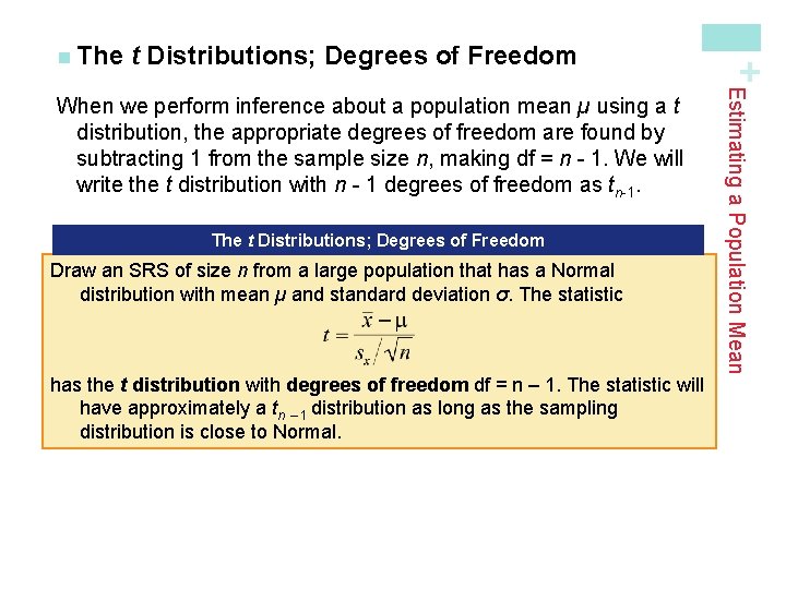
t Distributions; Degrees of Freedom The t Distributions; Degrees of Freedom Draw an SRS of size n from a large population that has a Normal distribution with mean µ and standard deviation σ. The statistic has the t distribution with degrees of freedom df = n – 1. The statistic will have approximately a tn – 1 distribution as long as the sampling distribution is close to Normal. Estimating a Population Mean When we perform inference about a population mean µ using a t distribution, the appropriate degrees of freedom are found by subtracting 1 from the sample size n, making df = n - 1. We will write the t distribution with n - 1 degrees of freedom as tn-1. + n The

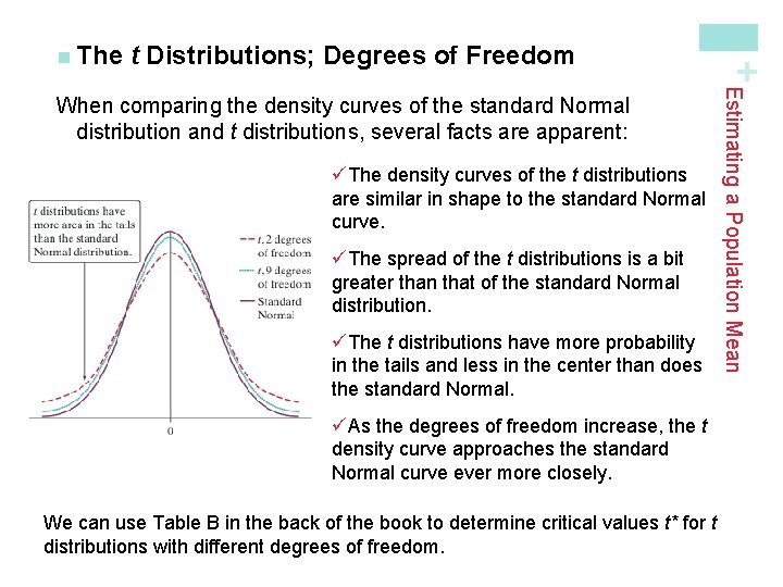
t Distributions; Degrees of Freedom üThe density curves of the t distributions are similar in shape to the standard Normal curve. üThe spread of the t distributions is a bit greater than that of the standard Normal distribution. üThe t distributions have more probability in the tails and less in the center than does the standard Normal. üAs the degrees of freedom increase, the t density curve approaches the standard Normal curve ever more closely. We can use Table B in the back of the book to determine critical values t* for t distributions with different degrees of freedom. Estimating a Population Mean When comparing the density curves of the standard Normal distribution and t distributions, several facts are apparent: + n The

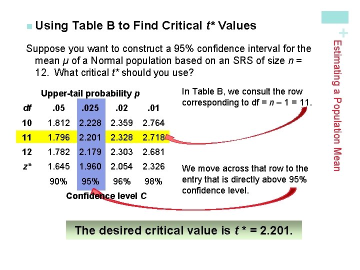
Table B to Find Critical t* Values Upper-tail probability p df . 05 . 02 . 01 10 1. 812 2. 228 2. 359 2. 764 11 1. 796 2. 201 2. 328 2. 718 12 1. 782 2. 179 2. 303 2. 681 z* 1. 645 1. 960 2. 054 2. 326 90% 95% 96% 98% Confidence level C In Table B, we consult the row corresponding to df = n – 1 = 11. We move across that row to the entry that is directly above 95% confidence level. The desired critical value is t * = 2. 201. Estimating a Population Mean Suppose you want to construct a 95% confidence interval for the mean µ of a Normal population based on an SRS of size n = 12. What critical t* should you use? + n Using

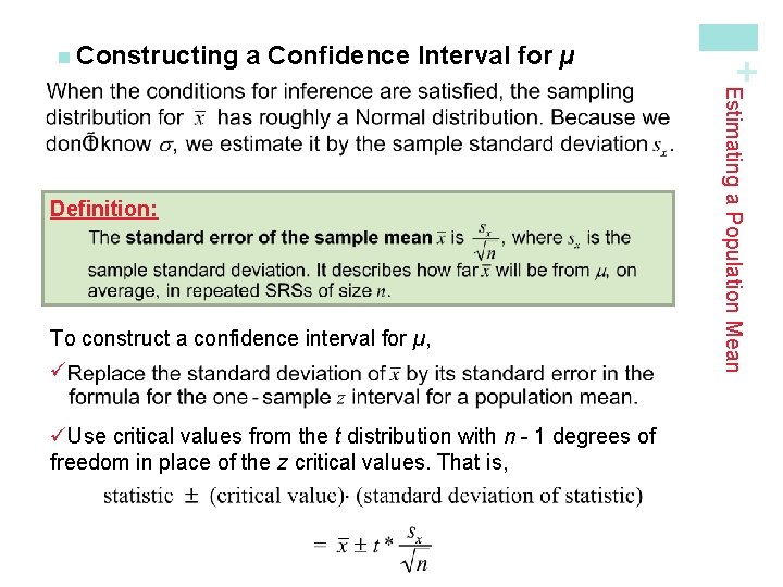
a Confidence Interval for µ To construct a confidence interval for µ, ü üUse critical values from the t distribution with n - 1 degrees of freedom in place of the z critical values. That is, Estimating a Population Mean Definition: + n Constructing

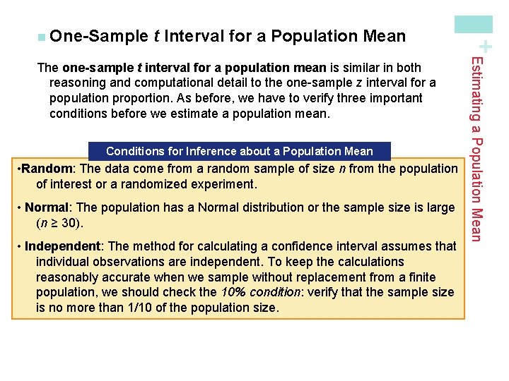
t Interval for a Population Mean Conditions The One-Sample for Inference t Interval about for aa. Population. Mean Choose an The SRSdata of size n from havingofunknown mean A level • Random: come fromaapopulation random sample size n from theµ. population C confidence for µ isexperiment. of interest or ainterval randomized • Normal: The population has a Normal distribution or the sample size is large (n ≥ 30). where t* is the critical value for the tn – 1 distribution. • Independent: The method for calculating a confidence interval assumes that Use this interval only when: individual observations are independent. To keep the calculations accurate wheniswe sample replacement from(na ≥finite (1) reasonably the population distribution Normal orwithout the sample size is large 30), population, we should check the 10% condition: verify that the sample size (2) the at least 10 population times as large is nopopulation more thanis 1/10 of the size. as the sample. Estimating a Population Mean The one-sample t interval for a population mean is similar in both reasoning and computational detail to the one-sample z interval for a population proportion. As before, we have to verify three important conditions before we estimate a population mean. + n One-Sample

Video Screen Tension PLAN: If the conditions are met, we can use a one-sample t interval to estimate µ. Random: We are told that the data come from a random sample of 20 screens from the population of all screens produced that day. Normal: Since the sample size is small (n < 30), we must check whether it’s reasonable to believe that the population distribution is Normal. Examine the distribution of the sample data. These graphs give no reason to doubt the Normality of the population Independent: Because we are sampling without replacement, we must check the 10% condition: we must assume that at least 10(20) = 200 video terminals were produced this day. Estimating a Population Mean Read the Example on page 508. STATE: We want to estimate the true mean tension µ of all the video terminals produced this day at a 90% confidence level. + n Example:

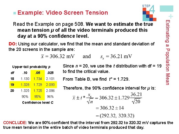
Video Screen Tension DO: Using our calculator, we find that the mean and standard deviation of the 20 screens in the sample are: df . 10 . 05 . 025 Since n = 20, we use the t distribution with df = 19 to find the critical value. 18 1. 130 1. 734 2. 101 From Table B, we find t* = 1. 729. 19 1. 328 1. 729 2. 093 20 1. 325 1. 725 2. 086 90% 95% 96% Upper-tail probability p Therefore, the 90% confidence interval for µ is: Estimating a Population Mean Read the Example on page 508. We want to estimate the true mean tension µ of all the video terminals produced this day at a 90% confidence level. + n Example: Confidence level C CONCLUDE: We are 90% confident that the interval from 292. 32 to 320. 32 m. V captures the true mean tension in the entire batch of video terminals produced that day.

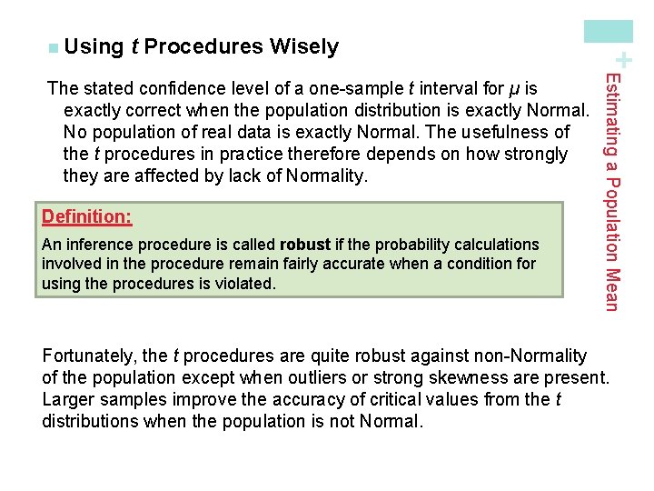
t Procedures Wisely Definition: An inference procedure is called robust if the probability calculations involved in the procedure remain fairly accurate when a condition for using the procedures is violated. Estimating a Population Mean The stated confidence level of a one-sample t interval for µ is exactly correct when the population distribution is exactly Normal. No population of real data is exactly Normal. The usefulness of the t procedures in practice therefore depends on how strongly they are affected by lack of Normality. + n Using Fortunately, the t procedures are quite robust against non-Normality of the population except when outliers or strong skewness are present. Larger samples improve the accuracy of critical values from the t distributions when the population is not Normal.

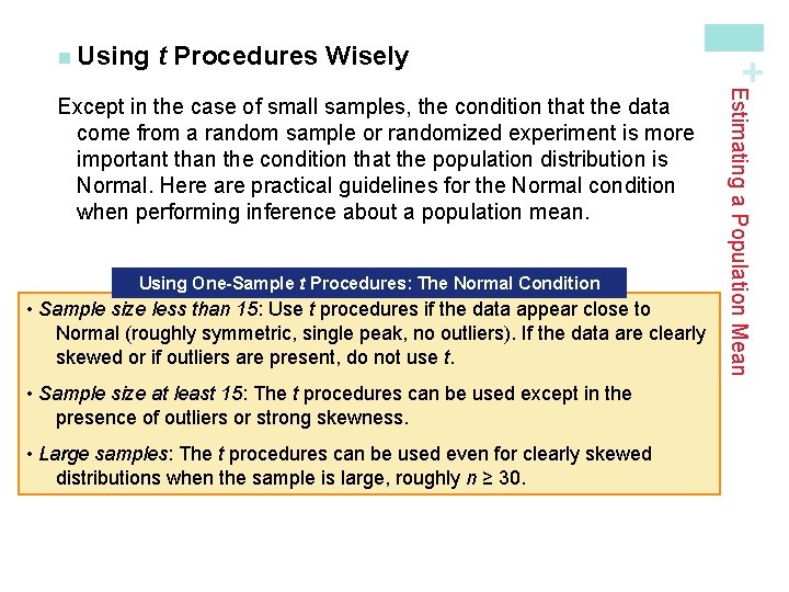
t Procedures Wisely Using One-Sample t Procedures: The Normal Condition • Sample size less than 15: Use t procedures if the data appear close to Normal (roughly symmetric, single peak, no outliers). If the data are clearly skewed or if outliers are present, do not use t. • Sample size at least 15: The t procedures can be used except in the presence of outliers or strong skewness. • Large samples: The t procedures can be used even for clearly skewed distributions when the sample is large, roughly n ≥ 30. Estimating a Population Mean Except in the case of small samples, the condition that the data come from a random sample or randomized experiment is more important than the condition that the population distribution is Normal. Here are practical guidelines for the Normal condition when performing inference about a population mean. + n Using

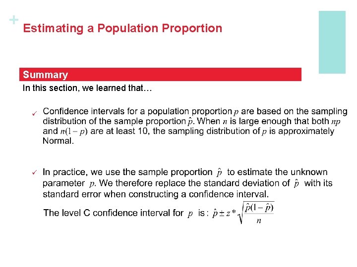
+ Estimating a Population Proportion Summary In this section, we learned that… ü ü

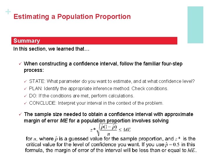
+ Estimating a Population Proportion Summary In this section, we learned that… ü ü When constructing a confidence interval, follow the familiar four-step process: ü STATE: What parameter do you want to estimate, and at what confidence level? ü PLAN: Identify the appropriate inference method. Check conditions. ü DO: If the conditions are met, perform calculations. ü CONCLUDE: Interpret your interval in the context of the problem. The sample size needed to obtain a confidence interval with approximate margin of error ME for a population proportion involves solving

+ Estimating a Population Mean Summary In this section, we learned that… ü Confidence intervals for the mean µ of a Normal population are based on the sample mean of an SRS. ü If we somehow know σ, we use the z critical value and the standard Normal distribution to help calculate confidence intervals. ü The sample size needed to obtain a confidence interval with approximate margin of error ME for a population mean involves solving ü In practice, we usually don’t know σ. Replace the standard deviation of the sampling distribution with the standard error and use the t distribution with n – 1 degrees of freedom (df).

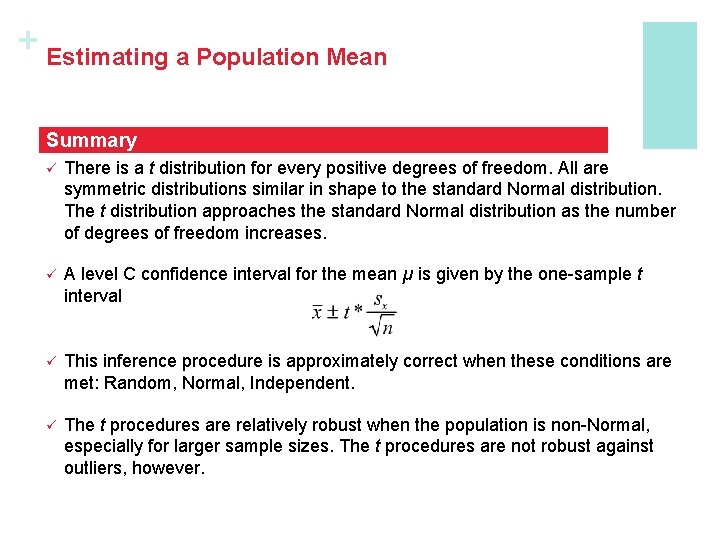
+ Estimating a Population Mean Summary ü There is a t distribution for every positive degrees of freedom. All are symmetric distributions similar in shape to the standard Normal distribution. The t distribution approaches the standard Normal distribution as the number of degrees of freedom increases. ü A level C confidence interval for the mean µ is given by the one-sample t interval ü This inference procedure is approximately correct when these conditions are met: Random, Normal, Independent. ü The t procedures are relatively robust when the population is non-Normal, especially for larger sample sizes. The t procedures are not robust against outliers, however.