Dynamic Causal Modelling for f MRI Rosalyn Moran

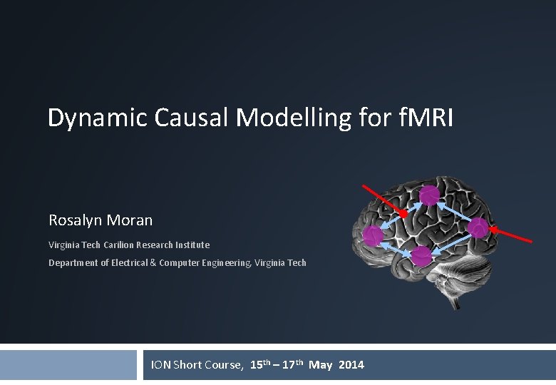
Dynamic Causal Modelling for f. MRI Rosalyn Moran Virginia Tech Carilion Research Institute Department of Electrical & Computer Engineering, Virginia Tech ION Short Course, 15 th – 17 th May 2014

Dynamic Causal Modelling DCM framework was introduced in 2003 for f. MRI by Karl Friston, Lee Harrison and Will Penny (Neuro. Image 19: 1273 -1302) part of the SPM software package >300 papers published 2

Overview Dynamic causal models (DCMs) § Basic idea § Neural level § Hemodynamic level § Parameter estimation, priors & inference Applications of DCM to f. MRI data § Attention to motion in the visual system § Modelling synesthesia § The Status Quo Bias 3

Overview Dynamic causal models (DCMs) § Basic idea § Neural level § Hemodynamic level § Parameter estimation, priors & inference Applications of DCM to f. MRI data § Attention to motion in the visual system § Modelling synesthesia § The Status Quo Bias 4

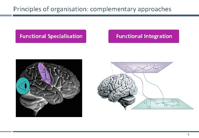
Principles of organisation: complementary approaches Functional Specialisation Functional Integration 5

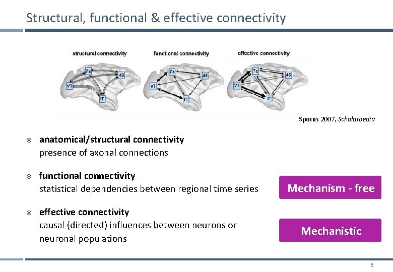
Structural, functional & effective connectivity Sporns 2007, Scholarpedia anatomical/structural connectivity presence of axonal connections functional connectivity statistical dependencies between regional time series effective connectivity causal (directed) influences between neurons or neuronal populations Mechanism - free Mechanistic 6

Functional vs Effective Connectivity Functional connectivity is defined in terms of statistical dependencies: an operational concept that underlies the detection of a functional connection, without any commitment to how that connection was caused - Assessing mutual information & testing for significant departures from zero - Simple assessment: patterns of correlations - Undirected or Directed Functional Connectivity eg. Granger Connectivity Effective connectivity is defined at the level of hidden neuronal states generating measurements. Effective connectivity is always directed and rests on an explicit (parameterised) model of causal influences — usually expressed in terms of difference (discrete time) or differential (continuous time) equations. - DCM - SEM

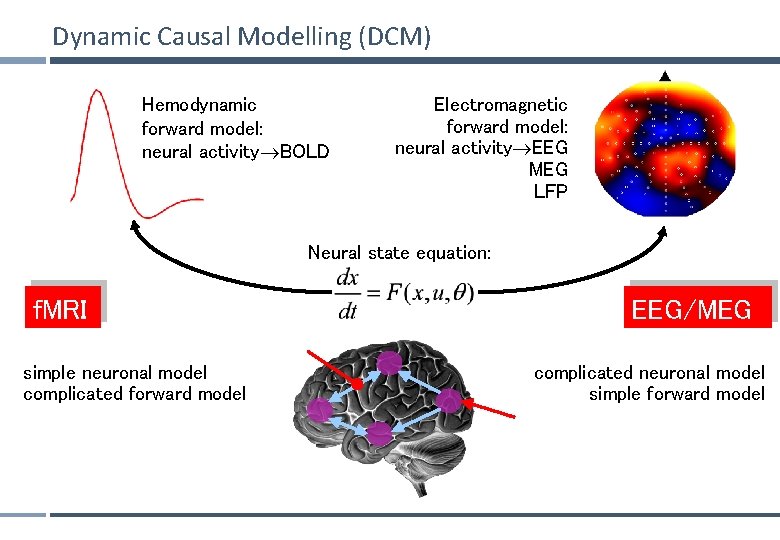
Dynamic Causal Modelling (DCM) Hemodynamic forward model: neural activity BOLD Electromagnetic forward model: neural activity EEG MEG LFP Neural state equation: f. MRI simple neuronal model complicated forward model EEG/MEG complicated neuronal model simple forward model

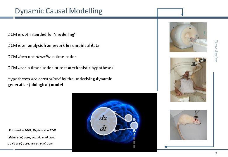
Dynamic Causal Modelling DCM is not intended for ‘modelling’ DCM does not describe a time series Time Series DCM is an analysis framework for empirical data DCM uses a times series to test mechanistic hypotheses Hypotheses are constrained by the underlying dynamic generative (biological) model Friston et al 2003; Stephan et al 2008 Kiebel et al, 2006; Garrido et al, 2007 David et al, 2006; Moran et al, 2007 9

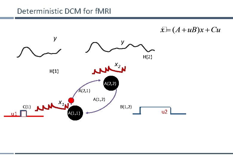
Deterministic DCM for f. MRI y y x 2 H{1} H{2} A(2, 2) A(2, 1) C(1) u 1 A(1, 2) x 1 B(1, 2) A(1, 1) u 2

Overview Dynamic causal models (DCMs) § Basic idea § Neural level § Hemodynamic level § Parameter estimation, priors & inference Applications of DCM to f. MRI data § Attention to motion in the visual system § Modelling synesthesia § The Status Quo Bias 11

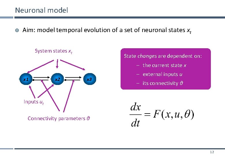
Neuronal model Aim: model temporal evolution of a set of neuronal states xt System states xt State changes are dependent on: – the current state x x 1 x 2 x 3 – external inputs u – its connectivity θ Inputs ut Connectivity parameters θ 12

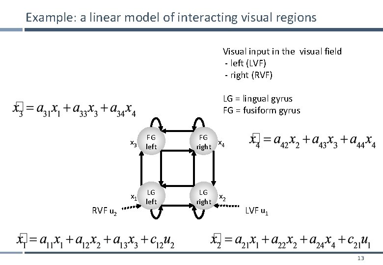
Example: a linear model of interacting visual regions Visual input in the visual field - left (LVF) - right (RVF) LG = lingual gyrus FG = fusiform gyrus x 3 left FG FG x right 4 LG left LG x right 2 x 1 RVF u 2 LVF u 1 13

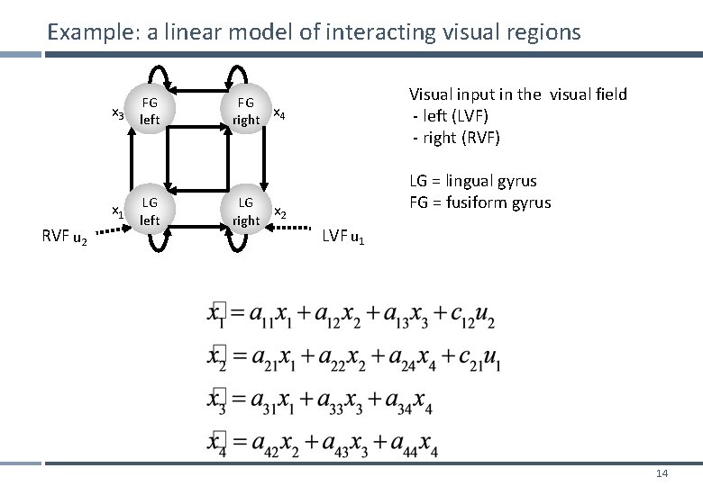
Example: a linear model of interacting visual regions x 3 x 1 RVF u 2 FG left LG left Visual input in the visual field - left (LVF) - right (RVF) FG x right 4 LG x right 2 LG = lingual gyrus FG = fusiform gyrus LVF u 1 14

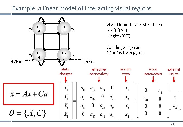
Example: a linear model of interacting visual regions x 3 x 1 RVF u 2 FG left LG left Visual input in the visual field - left (LVF) - right (RVF) FG x right 4 LG x right 2 state changes LG = lingual gyrus FG = fusiform gyrus LVF u 1 effective connectivity system state input parameters external inputs 15

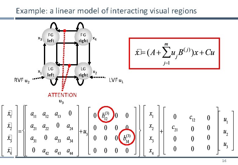
Example: a linear model of interacting visual regions x 3 left FG FG x right 4 LG left LG x right 2 x 1 RVF u 2 LVF u 1 ATTENTION u 3 16

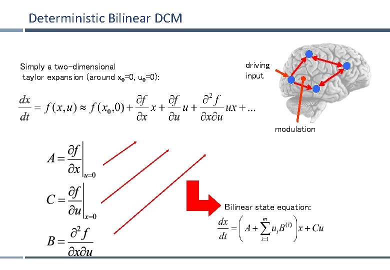
Deterministic Bilinear DCM Simply a two-dimensional taylor expansion (around x 0=0, u 0=0): driving input modulation Bilinear state equation:

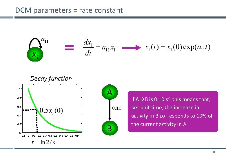
DCM parameters = rate constant x 1 Decay function 1 0. 8 A 0. 10 0. 6 0. 4 0. 2 0 B If A B is 0. 10 s-1 this means that, per unit time, the increase in activity in B corresponds to 10% of the current activity in A -0. 1 0. 2 0. 3 0. 4 0. 5 0. 6 0. 7 0. 8 0. 9 18

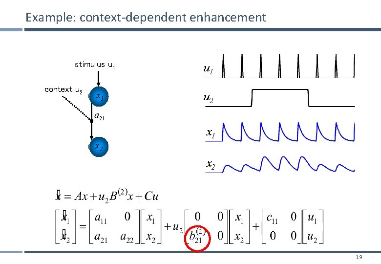
Example: context-dependent enhancement stimulus u 1 context u 2 x 1 x 2 u 1 u 2 x 1 x 2 19

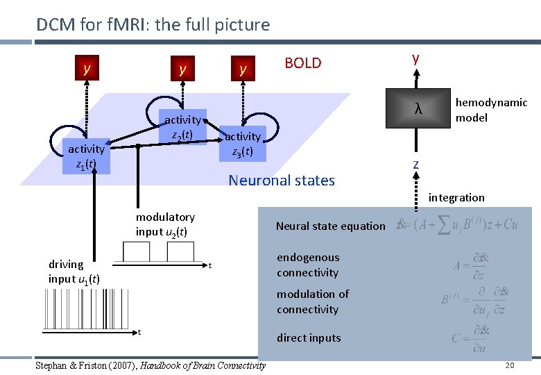
DCM for f. MRI: the full picture y y y activity z 3(t) Neuronal states modulatory input u 2(t) driving input u 1(t) y λ activity z 2(t) activity z 1(t) BOLD hemodynamic model z integration Neural state equation t endogenous connectivity modulation of connectivity t Stephan & Friston (2007), Handbook of Brain Connectivity direct inputs 20

Overview Dynamic causal models (DCMs) § Basic idea § Neural level § Hemodynamic level § Parameter estimation, priors & inference Applications of DCM to f. MRI data § Attention to motion in the visual system § Modelling synesthesia § The Status-Quo Bias 21

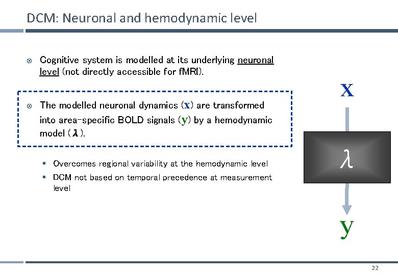
DCM: Neuronal and hemodynamic level Cognitive system is modelled at its underlying neuronal level (not directly accessible for f. MRI). The modelled neuronal dynamics (x) are transformed into area-specific BOLD signals (y) by a hemodynamic model (λ). § Overcomes regional variability at the hemodynamic level § DCM not based on temporal precedence at measurement level x λ y 22

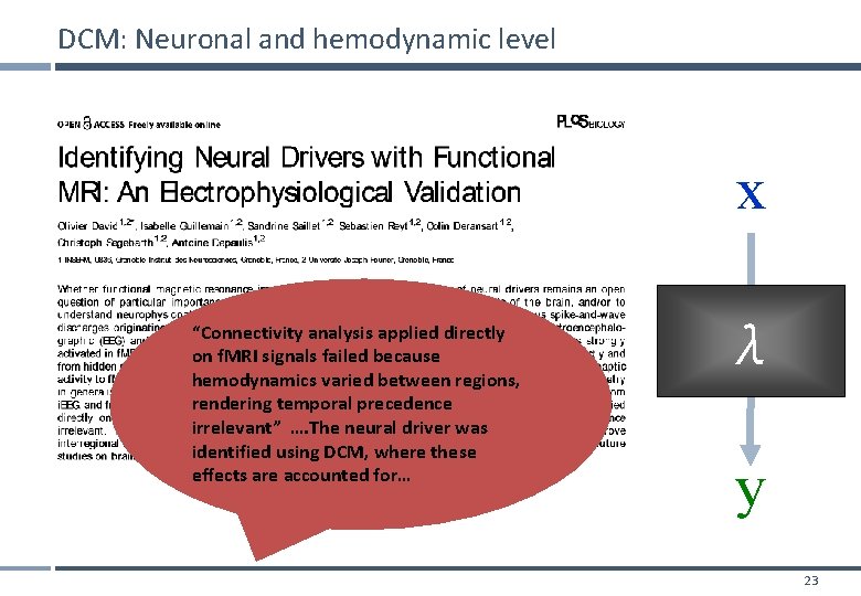
DCM: Neuronal and hemodynamic level x “Connectivity analysis applied directly on f. MRI signals failed because hemodynamics varied between regions, rendering temporal precedence irrelevant” …. The neural driver was identified using DCM, where these effects are accounted for… λ y 23

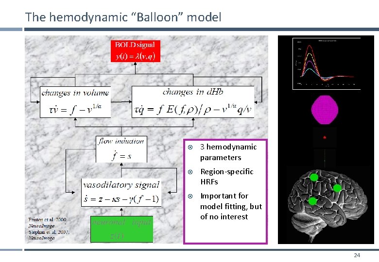
The hemodynamic “Balloon” model 3 hemodynamic parameters Region-specific HRFs Important for model fitting, but of no interest 24

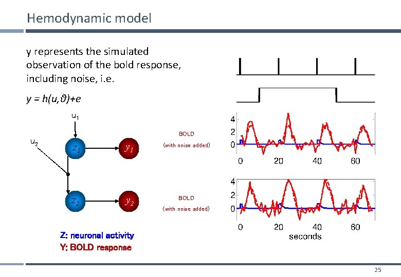
Hemodynamic model y represents the simulated observation of the bold response, including noise, i. e. y = h(u, θ)+e u 1 u 2 BOLD z 1 y 1 (with noise added) z 2 y 2 BOLD (with noise added) Z: neuronal activity Y: BOLD response 25

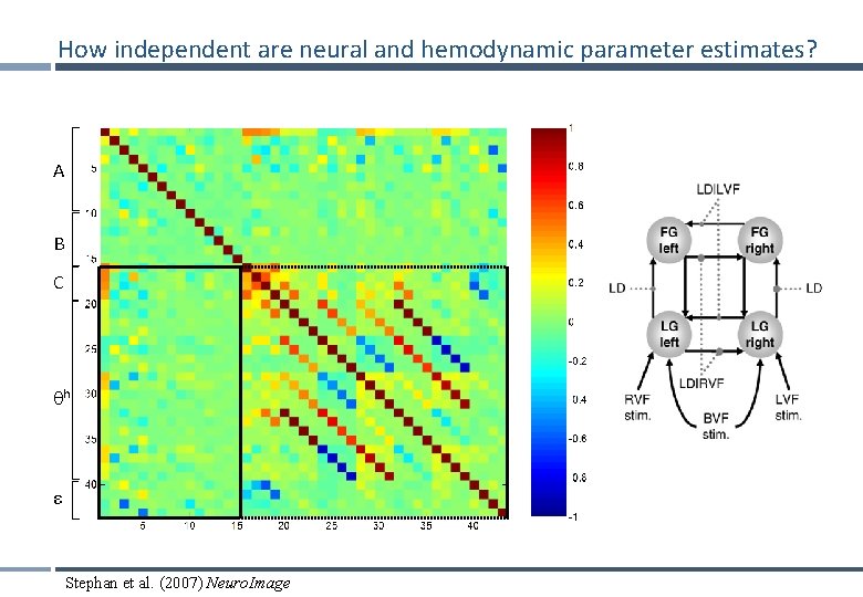
How independent are neural and hemodynamic parameter estimates? A B C h ε Stephan et al. (2007) Neuro. Image

Overview Dynamic causal models (DCMs) § Basic idea § Neural level § Hemodynamic level § Parameter estimation, priors & inference Applications of DCM to f. MRI data § Attention to motion in the visual system § Modelling synesthesia § The Status-Quo Bias 27

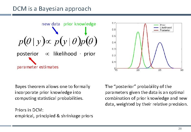
DCM is a Bayesian approach new data prior knowledge posterior likelihood ∙ prior parameter estimates Bayes theorem allows one to formally incorporate prior knowledge into computing statistical probabilities. Priors in DCM: empirical, principled & shrinkage priors The “posterior” probability of the parameters given the data is an optimal combination of prior knowledge and new data, weighted by their relative precision. 28

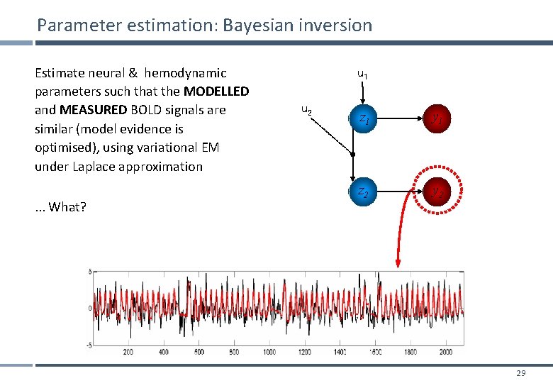
Parameter estimation: Bayesian inversion Estimate neural & hemodynamic parameters such that the MODELLED and MEASURED BOLD signals are similar (model evidence is optimised), using variational EM under Laplace approximation. . . What? u 1 u 2 z 1 y 1 z 2 y 2 29

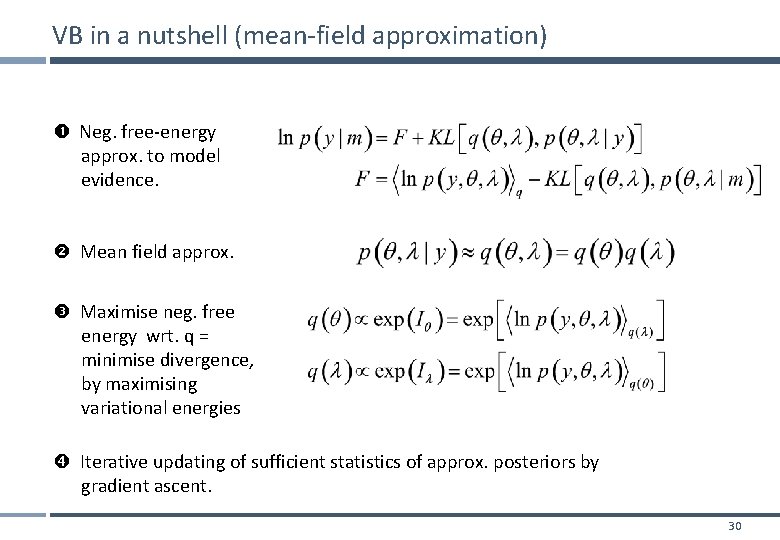
VB in a nutshell (mean-field approximation) Neg. free-energy approx. to model evidence. Mean field approx. Maximise neg. free energy wrt. q = minimise divergence, by maximising variational energies Iterative updating of sufficient statistics of approx. posteriors by gradient ascent. 30

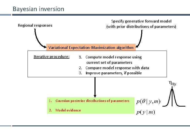
Bayesian inversion Specify generative forward model (with prior distributions of parameters) Regional responses Variational Expectation-Maximization algorithm Iterative procedure: 1. Compute model response using current set of parameters 2. Compare model response with data 3. Improve parameters, if possible ηθ|y 1. Gaussian posterior distributions of parameters 2. Model evidence

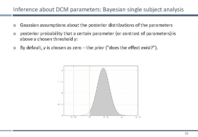
Inference about DCM parameters: Bayesian single subject analysis Gaussian assumptions about the posterior distributions of the parameters posterior probability that a certain parameter (or contrast of parameters) is above a chosen threshold γ: By default, γ is chosen as zero – the prior ("does the effect exist? "). 32

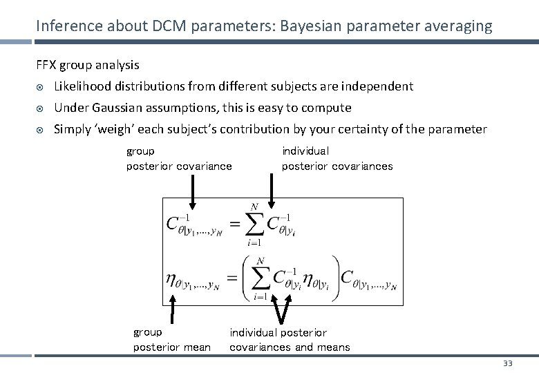
Inference about DCM parameters: Bayesian parameter averaging FFX group analysis Likelihood distributions from different subjects are independent Under Gaussian assumptions, this is easy to compute Simply ‘weigh’ each subject’s contribution by your certainty of the parameter group posterior covariance group posterior mean individual posterior covariances and means 33

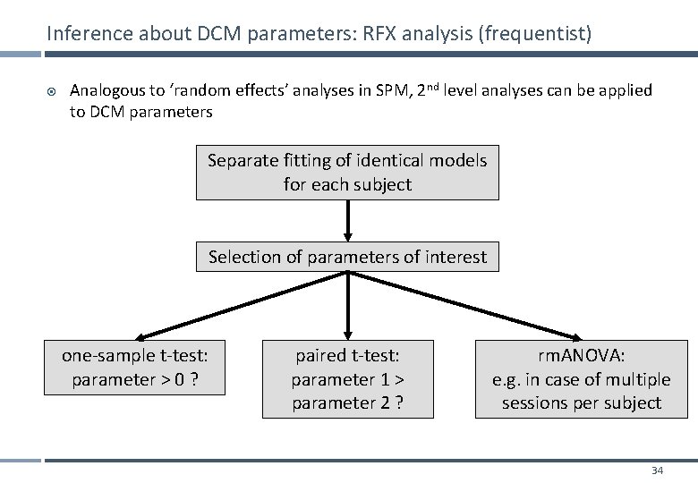
Inference about DCM parameters: RFX analysis (frequentist) Analogous to ‘random effects’ analyses in SPM, 2 nd level analyses can be applied to DCM parameters Separate fitting of identical models for each subject Selection of parameters of interest one-sample t-test: parameter > 0 ? paired t-test: parameter 1 > parameter 2 ? rm. ANOVA: e. g. in case of multiple sessions per subject 34

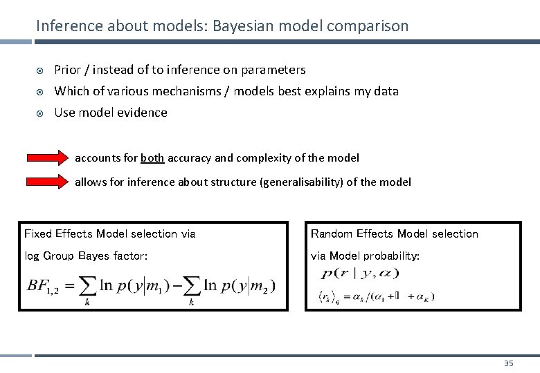
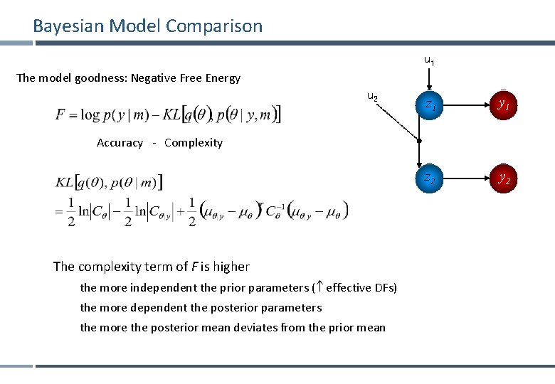
Inference about models: Bayesian model comparison Prior / instead of to inference on parameters Which of various mechanisms / models best explains my data Use model evidence accounts for both accuracy and complexity of the model allows for inference about structure (generalisability) of the model Fixed Effects Model selection via Random Effects Model selection log Group Bayes factor: via Model probability: 35

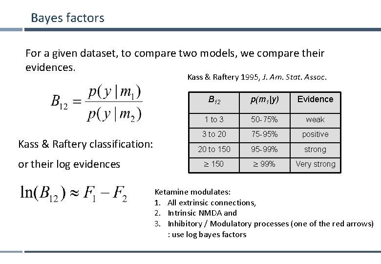
Bayes factors For a given dataset, to compare two models, we compare their evidences. Kass & Raftery 1995, J. Am. Stat. Assoc. Kass & Raftery classification: or their log evidences B 12 p(m 1|y) Evidence 1 to 3 50 -75% weak 3 to 20 75 -95% positive 20 to 150 95 -99% strong 150 99% Very strong Ketamine modulates: 1. All extrinsic connections, 2. Intrinsic NMDA and 3. Inhibitory / Modulatory processes (one of the red arrows) : use log bayes factors

Bayesian Model Comparison u 1 The model goodness: Negative Free Energy u 2 z 1 y 1 z 2 y 2 Accuracy - Complexity The complexity term of F is higher the more independent the prior parameters ( effective DFs) the more dependent the posterior parameters the more the posterior mean deviates from the prior mean

Overview Dynamic causal models (DCMs) § Basic idea § Neural level § Hemodynamic level § Parameter estimation, priors & inference Applications of DCM to f. MRI data § Attention to motion in the visual system § Modelling synesthesia § The Status-Quo Bias 38

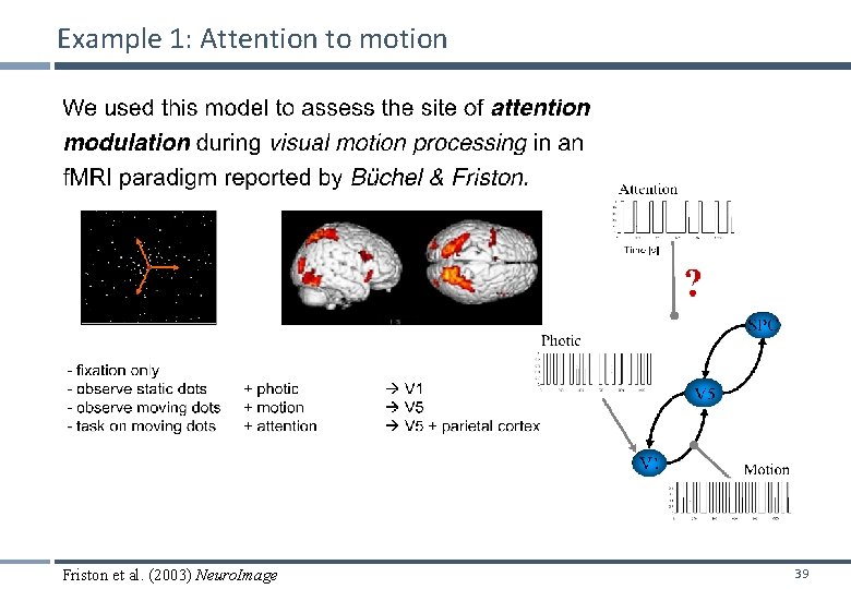
Example 1: Attention to motion Friston et al. (2003) Neuro. Image 39

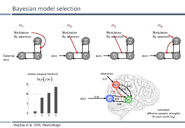
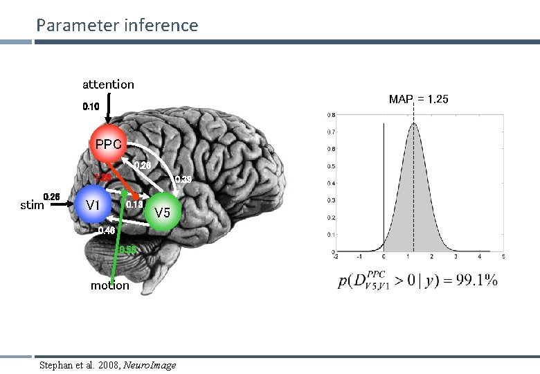
Bayesian model selection m 1 m 2 Modulation By attention V 1 V 5 m 4 Modulation By attention PPC External stim m 3 stim V 1 V 5 Modulation By attention PPC stim V 1 V 5 attention models marginal likelihood 0. 10 PPC 0. 39 0. 26 1. 25 stim 0. 26 V 1 0. 13 V 5 0. 46 estimated effective synaptic strengths for best model (m 4) Stephan et al. 2008, Neuro. Image

Parameter inference attention MAP = 1. 25 0. 10 PPC 0. 26 1. 25 0. 26 stim V 1 0. 39 0. 13 V 5 0. 46 0. 50 motion Stephan et al. 2008, Neuro. Image

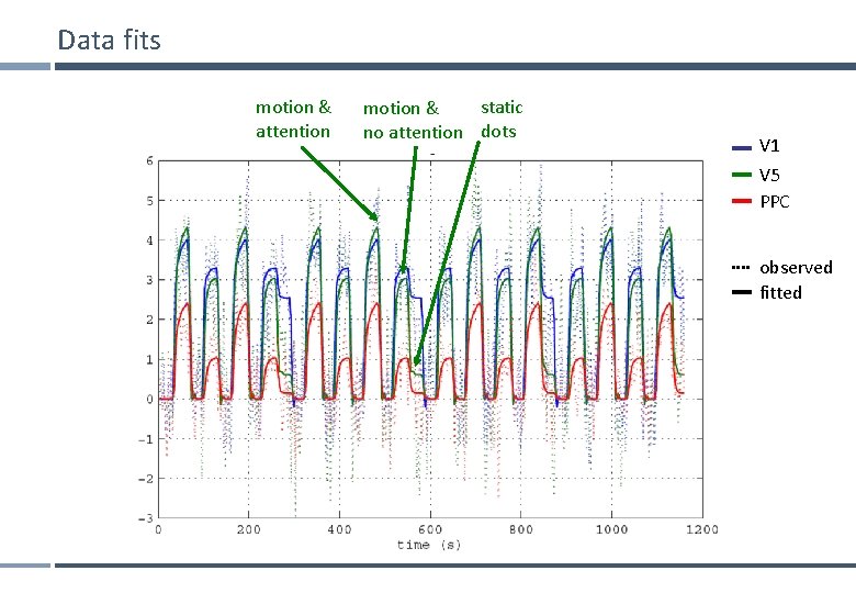
Data fits motion & attention static motion & no attention dots V 1 V 5 PPC observed fitted

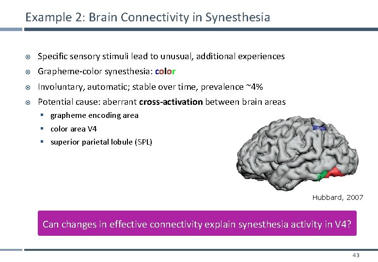
Example 2: Brain Connectivity in Synesthesia Specific sensory stimuli lead to unusual, additional experiences Grapheme-color synesthesia: color Involuntary, automatic; stable over time, prevalence ~4% Potential cause: aberrant cross-activation between brain areas § grapheme encoding area § color area V 4 § superior parietal lobule (SPL) Hubbard, 2007 Can changes in effective connectivity explain synesthesia activity in V 4? 43

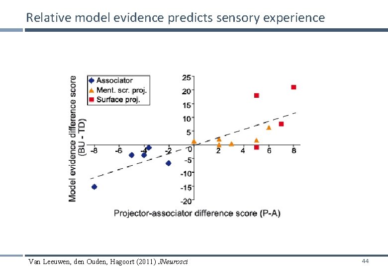
Relative model evidence predicts sensory experience Van Leeuwen, den Ouden, Hagoort (2011) JNeurosci 44

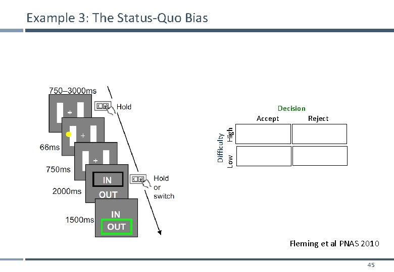
Example 3: The Status-Quo Bias Difficulty Low High Decision Accept Reject Fleming et al PNAS 2010 45

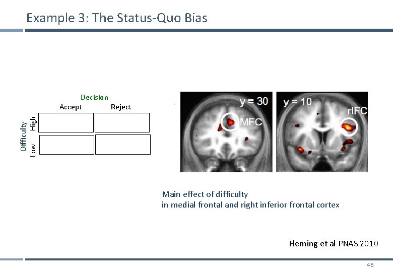
Example 3: The Status-Quo Bias Difficulty Low High Decision Accept Reject Main effect of difficulty in medial frontal and right inferior frontal cortex Fleming et al PNAS 2010 46

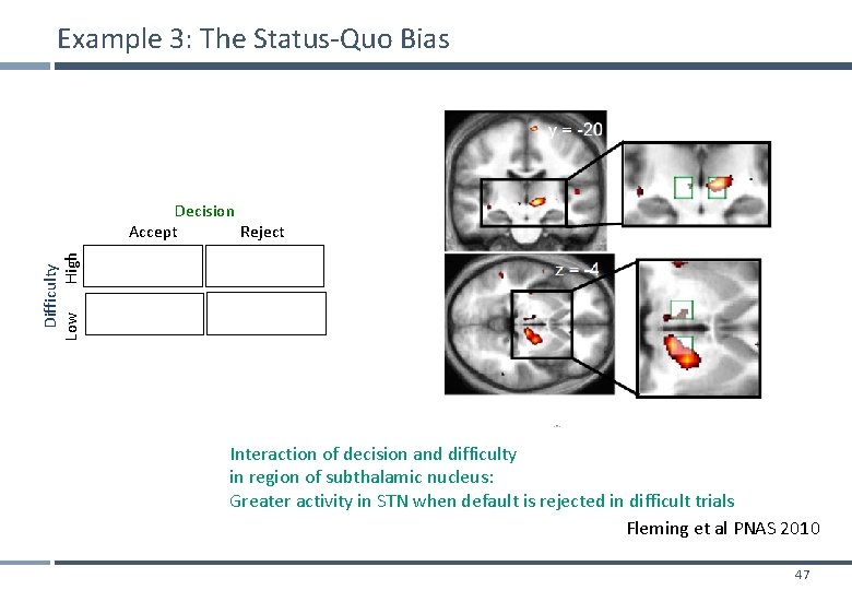
Example 3: The Status-Quo Bias Difficulty Low High Decision Accept Reject Interaction of decision and difficulty in region of subthalamic nucleus: Greater activity in STN when default is rejected in difficult trials Fleming et al PNAS 2010 47

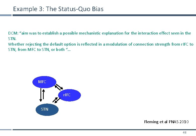
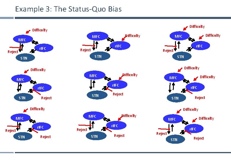
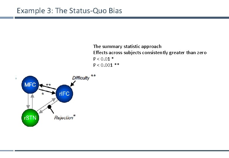
Example 3: The Status-Quo Bias DCM: “aim was to establish a possible mechanistic explanation for the interaction effect seen in the STN. Whether rejecting the default option is reflected in a modulation of connection strength from r. IFC to STN, from MFC to STN, or both “… MFC r. IFC STN Fleming et al PNAS 2010 48

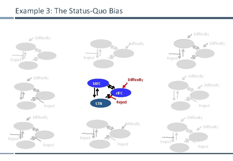
Example 3: The Status-Quo Bias Difficulty r. IFC Reject Difficulty MFC r. IFC Reject STN Difficulty MFC STN Reject r. IFC Reject STN Difficulty MFC Reject Difficulty MFC r. IFC STN r. IFC Reject STN Difficulty MFC r. IFC Reject STN Reject

Example 3: The Status-Quo Bias Difficulty MFC r. IFC Reject STN Difficulty STN Reject r. IFC Reject STN Difficulty MFC Reject Difficulty MFC r. IFC STN Difficulty MFC r. IFC Reject STN Reject

Example 3: The Status-Quo Bias The summary statistic approach Effects across subjects consistently greater than zero P < 0. 01 * P < 0. 001 **

Final note 1: The evolution of DCM in SPM DCM is not one specific model, but a framework for Bayesian inversion of dynamic system models The default implementation in SPM is evolving over time § better numerical routines for inversion § change in priors to cover new variants (e. g. , stochastic DCMs, endogenous DCMs etc. ) To enable replication of your results, you should ideally state which SPM version you are using when publishing papers. 52

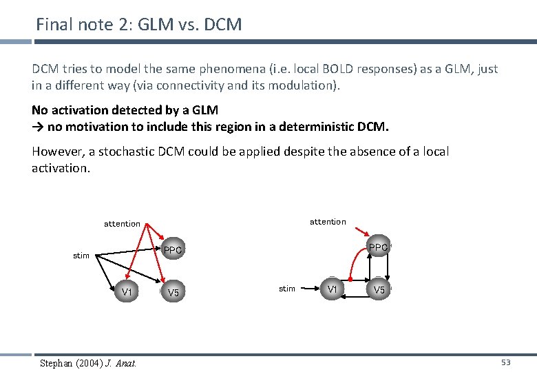
Final note 2: GLM vs. DCM tries to model the same phenomena (i. e. local BOLD responses) as a GLM, just in a different way (via connectivity and its modulation). No activation detected by a GLM → no motivation to include this region in a deterministic DCM. However, a stochastic DCM could be applied despite the absence of a local activation. attention PPC stim V 1 Stephan (2004) J. Anat. V 5 stim V 1 V 5 53

Other exciting developments • • Nonlinear DCM for f. MRI: Could connectivity changes be mediated by another region? (Stephan et al. 2008) Clustering DCM parameters: Classify patients, or even find new sub-categories (Brodersen et al. 2011 Neuroimage) • • • Embedding computational models in DCMs: DCM can be used to make inferences on parametric designs like SPM (den Ouden et al. 2010, J Neurosci. ) Integrating tractography and DCM: Prior variance is a good way to embed other forms of information, test validity (Stephan et al. 2009, Neuro. Image) Stochastic DCM: Model resting state studies / background fluctuations (Li et al. 2011 Neuroimage, Daunizeau et al. Physica D 2009) 54

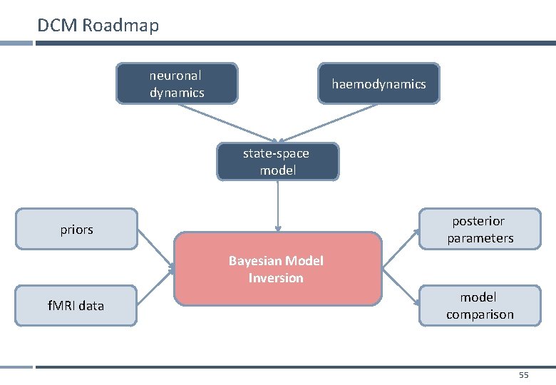
DCM Roadmap neuronal dynamics haemodynamics state-space model posterior parameters priors Bayesian Model Inversion f. MRI data model comparison 55

Some useful references • 10 Simple Rules for DCM (2010). Stephan et al. Neuro. Image 52. • The first DCM paper: Dynamic Causal Modelling (2003). Friston et al. Neuro. Image 19: 12731302. • Physiological validation of DCM for f. MRI: Identifying neural drivers with functional MRI: an electrophysiological validation (2008). David et al. PLo. S Biol. 6 2683– 2697 • Hemodynamic model: Comparing hemodynamic models with DCM (2007). Stephan et al. Neuro. Image 38: 387 -401 • Nonlinear DCM: Nonlinear Dynamic Causal Models for FMRI (2008). Stephan et al. Neuro. Image 42: 649 -662 • Two-state DCM: Dynamic causal modelling for f. MRI: A two-state model (2008). Marreiros et al. Neuro. Image 39: 269 -278 • Stochastic DCM: Generalised filtering and stochastic DCM for f. MRI (2011). Li et al. Neuro. Image 58: 442 -457. • Bayesian model comparison: Comparing families of dynamic causal models (2010). Penny et al. PLo. S Comput Biol. 6(3): e 1000709. 56

Thank you 57

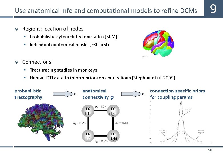
Use anatomical info and computational models to refine DCMs 9 Regions: location of nodes § Probabilistic cytoarchitectonic atlas (SPM) § Individual anatomical masks (FSL first) Connections § Tract tracing studies in monkeys § Human DTI data to inform priors on connections (Stephan et al. 2009) probabilistic tractography anatomical connectivity FG left FG right LG left LG right connection-specific priors for coupling params 58

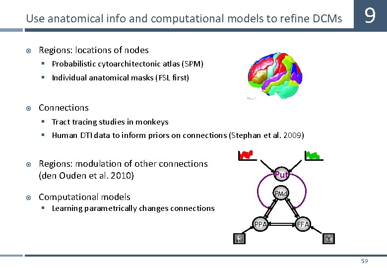
Use anatomical info and computational models to refine DCMs 9 Regions: locations of nodes § Probabilistic cytoarchitectonic atlas (SPM) § Individual anatomical masks (FSL first) Connections § Tract tracing studies in monkeys § Human DTI data to inform priors on connections (Stephan et al. 2009) Regions: modulation of other connections (den Ouden et al. 2010) Put PMd Computational models § Learning parametrically changes connections PPA FFA 59