Spatial Statistics and Analysis Methods for GEOG 104

Spatial Statistics and Analysis Methods (for GEOG 104 class). n Provided by Dr. An Li, San Diego State University. 1

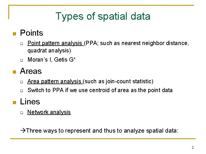
Types of spatial data n Points q q n n Point pattern analysis (PPA; such as nearest neighbor distance, quadrat analysis) Moran’s I, Getis G* Areas q Area pattern analysis (such as join-count statistic) q Switch to PPA if we use centroid of area as the point data Lines q Network analysis Three ways to represent and thus to analyze spatial data: 2

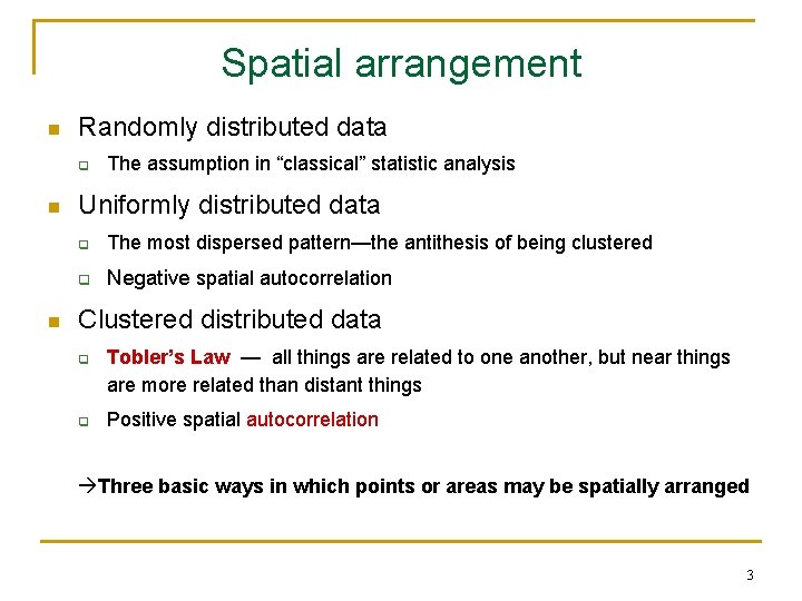
Spatial arrangement n Randomly distributed data q n n The assumption in “classical” statistic analysis Uniformly distributed data q The most dispersed pattern—the antithesis of being clustered q Negative spatial autocorrelation Clustered distributed data q q Tobler’s Law — all things are related to one another, but near things are more related than distant things Positive spatial autocorrelation Three basic ways in which points or areas may be spatially arranged 3

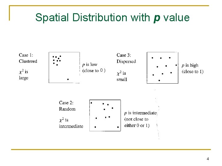
Spatial Distribution with p value 0) 4

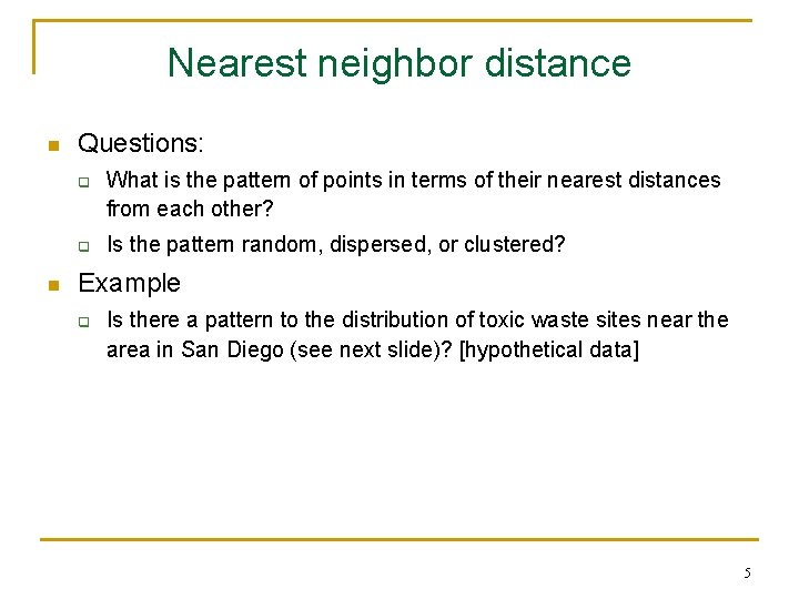
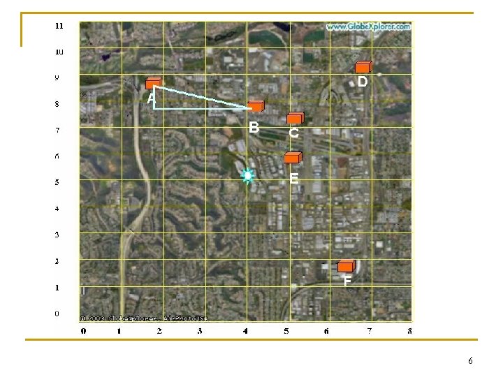
Nearest neighbor distance n Questions: q q n What is the pattern of points in terms of their nearest distances from each other? Is the pattern random, dispersed, or clustered? Example q Is there a pattern to the distribution of toxic waste sites near the area in San Diego (see next slide)? [hypothetical data] 5

6

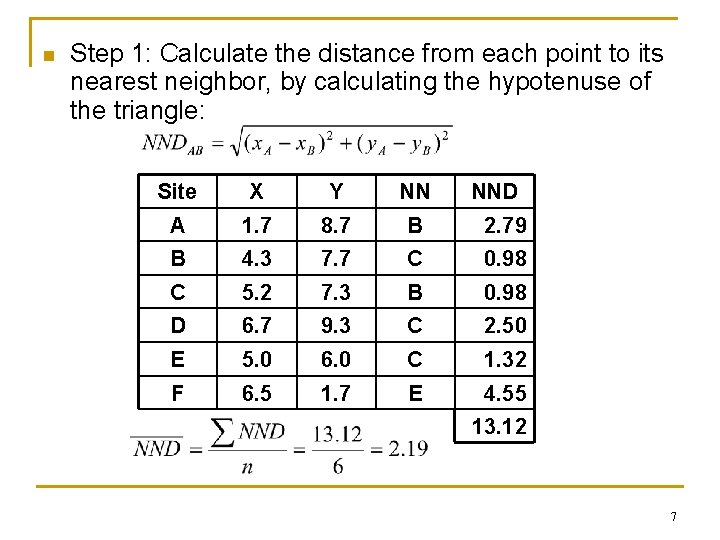
n Step 1: Calculate the distance from each point to its nearest neighbor, by calculating the hypotenuse of the triangle: Site X Y NN NND A 1. 7 8. 7 B 2. 79 B 4. 3 7. 7 C 0. 98 C 5. 2 7. 3 B 0. 98 D 6. 7 9. 3 C 2. 50 E 5. 0 6. 0 C 1. 32 F 6. 5 1. 7 E 4. 55 13. 12 7

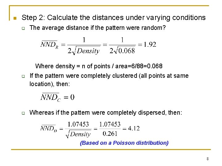
n Step 2: Calculate the distances under varying conditions q The average distance if the pattern were random? Where density = n of points / area=6/88=0. 068 q q If the pattern were completely clustered (all points at same location), then: Whereas if the pattern were completely dispersed, then: (Based on a Poisson distribution) 8

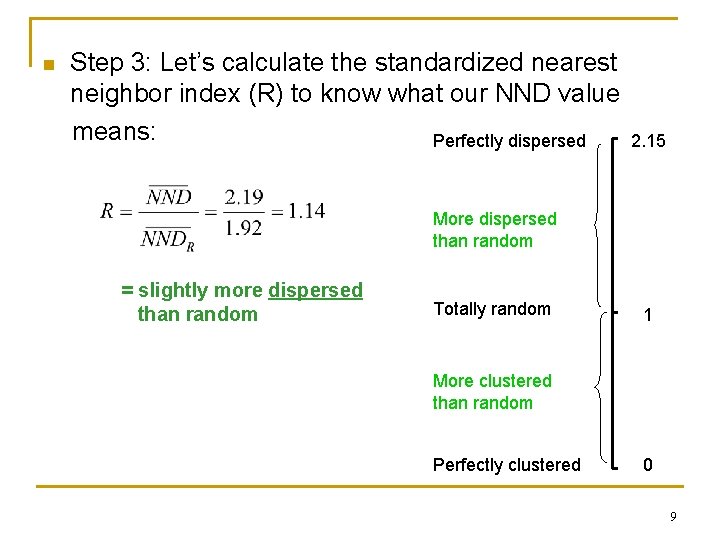
n Step 3: Let’s calculate the standardized nearest neighbor index (R) to know what our NND value means: Perfectly dispersed 2. 15 More dispersed than random = slightly more dispersed than random Totally random 1 More clustered than random Perfectly clustered 0 9

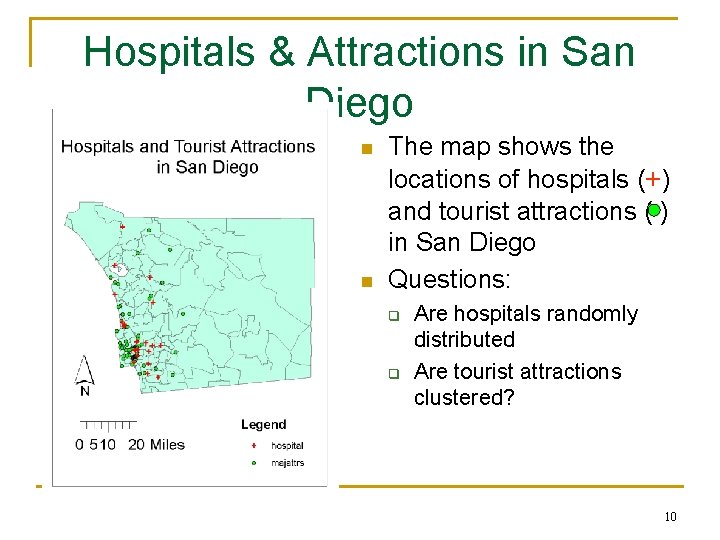
Hospitals & Attractions in San Diego n n The map shows the locations of hospitals (+) and tourist attractions ( ) in San Diego Questions: q q Are hospitals randomly distributed Are tourist attractions clustered? 10

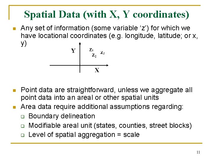
Spatial Data (with X, Y coordinates) n Any set of information (some variable ‘z’) for which we have locational coordinates (e. g. longitude, latitude; or x, y) n Point data are straightforward, unless we aggregate all point data into an areal or other spatial units Area data require additional assumptions regarding: q Boundary delineation q Modifiable areal unit (states, counties, street blocks) q Level of spatial aggregation = scale n 11

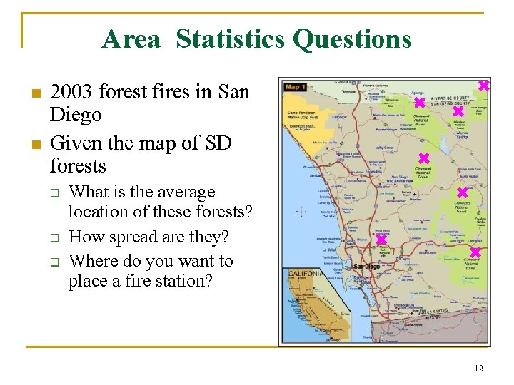
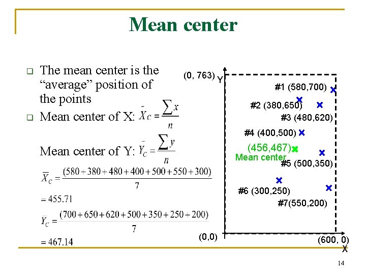
Area Statistics Questions n n 2003 forest fires in San Diego Given the map of SD forests q q q What is the average location of these forests? How spread are they? Where do you want to place a fire station? 12

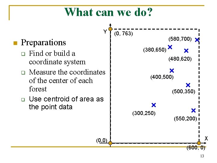
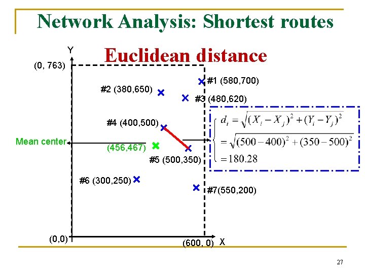
What can we do? Y n Preparations q q q Find or build a coordinate system Measure the coordinates of the center of each forest Use centroid of area as the point data (0, 763) (580, 700) (380, 650) (480, 620) (400, 500) (500, 350) (300, 250) (550, 200) X (0, 0) (600, 0) 13

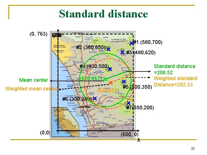
Mean center q q The mean center is the “average” position of the points Mean center of X: (0, 763) Y #1 (580, 700) #2 (380, 650) #3 (480, 620) #4 (400, 500) (456, 467) Mean center of Y: Mean center #5 (500, 350) #6 (300, 250) #7(550, 200) (0, 0) (600, 0) X 14

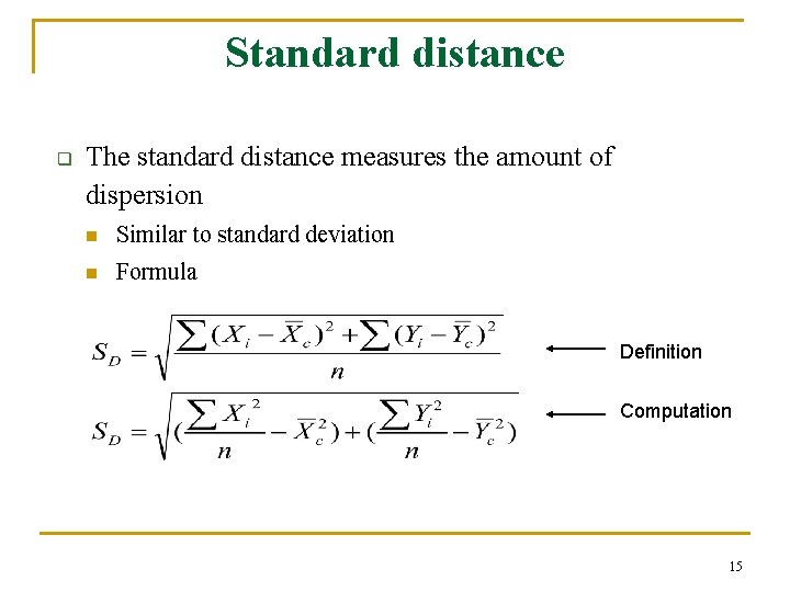
Standard distance q The standard distance measures the amount of dispersion n Similar to standard deviation n Formula Definition Computation 15

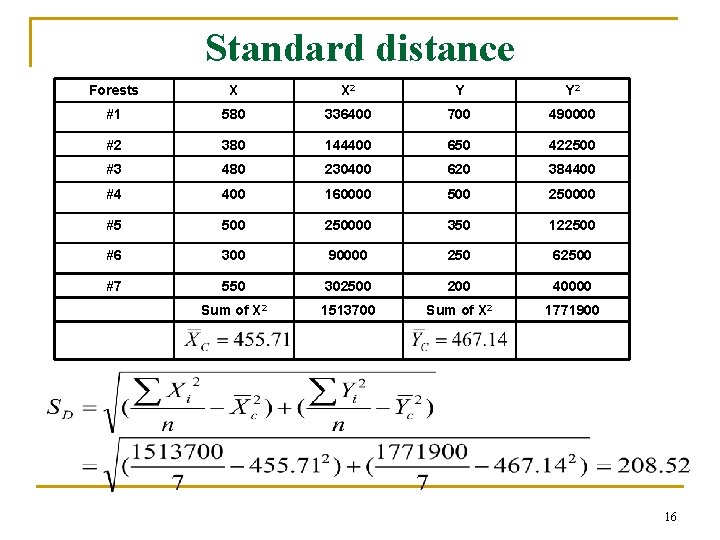
Standard distance Forests X X 2 Y Y 2 #1 580 336400 700 490000 #2 380 144400 650 422500 #3 480 230400 620 384400 #4 400 160000 500 250000 #5 500 250000 350 122500 #6 300 90000 250 62500 #7 550 302500 200 40000 Sum of X 2 1513700 Sum of X 2 1771900 16

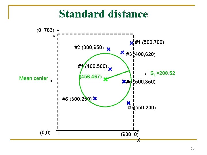
Standard distance (0, 763) Y #2 (380, 650) #1 (580, 700) #3 (480, 620) #4 (400, 500) Mean center (456, 467) SD=208. 52 #5 (500, 350) #6 (300, 250) #7(550, 200) (0, 0) (600, 0) X 17

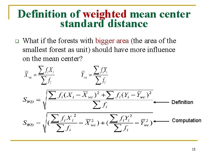
Definition of weighted mean center standard distance q What if the forests with bigger area (the area of the smallest forest as unit) should have more influence on the mean center? Definition Computation 18

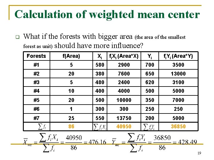
Calculation of weighted mean center q What if the forests with bigger area (the area of the smallest forest as unit) should have more influence? Forests f(Area) Xi fi. Xi (Area*X) Yi fi. Yi (Area*Y) #1 5 580 2900 700 3500 #2 20 380 7600 650 13000 #3 5 480 2400 620 3100 #4 10 4000 5000 #5 20 500 10000 350 7000 #6 1 300 250 #7 25 550 13750 200 5000 86 40950 36850 19

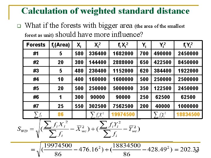
Calculation of weighted standard distance q What if the forests with bigger area (the area of the smallest forest as unit) should have more influence? Forests fi(Area) #1 5 580 336400 1682000 700 490000 2450000 #2 20 380 144400 2888000 650 422500 8450000 #3 5 480 230400 1152000 620 384400 1922000 #4 10 400 1600000 500 2500000 #5 20 500 25000000 350 122500 2450000 #6 1 300 #7 25 550 302500 86 Xi Xi 2 90000 fi Xi 2 Yi Yi 2 fi. Yi 2 90000 250 62500 7562500 200 40000 1000000 19974500 18834500 20

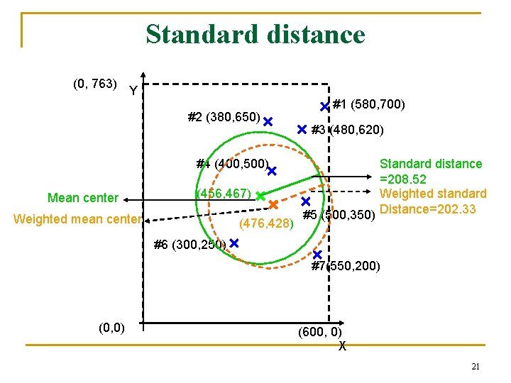
Standard distance (0, 763) Y #2 (380, 650) #4 (400, 500) Mean center (456, 467) Weighted mean center (476, 428) #1 (580, 700) #3 (480, 620) Standard distance =208. 52 Weighted standard #5 (500, 350) Distance=202. 33 #6 (300, 250) #7(550, 200) (0, 0) (600, 0) X 21

Standard distance (0, 763) Y #2 (380, 650) #4 (400, 500) Mean center (456, 467) Weighted mean center (476, 428) #1 (580, 700) #3 (480, 620) Standard distance =208. 52 Weighted standard #5 (500, 350) Distance=202. 33 #6 (300, 250) #7(550, 200) (0, 0) (600, 0) X 22

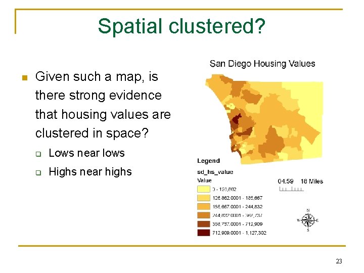
Spatial clustered? n Given such a map, is there strong evidence that housing values are clustered in space? q Lows near lows q Highs near highs 23

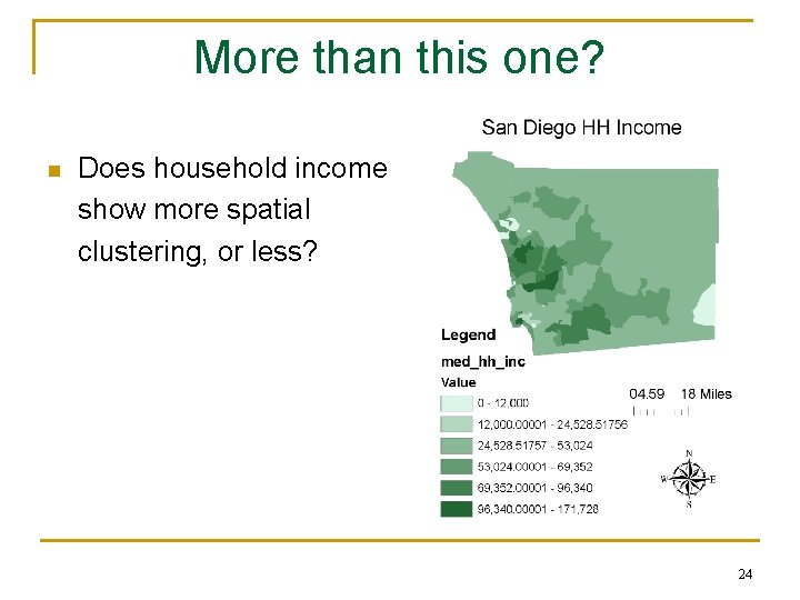
More than this one? n Does household income show more spatial clustering, or less? 24

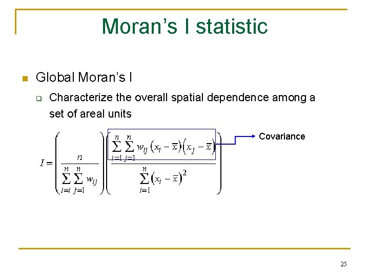
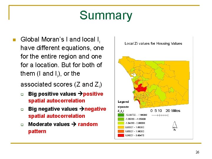
Moran’s I statistic n Global Moran’s I q Characterize the overall spatial dependence among a set of areal units Covariance 25

Summary n Global Moran’s I and local Ii have different equations, one for the entire region and one for a location. But for both of them (I and Ii), or the associated scores (Z and Zi) q q q Big positive values positive spatial autocorrelation Big negative values negative spatial autocorrelation Moderate values random pattern 26

Network Analysis: Shortest routes Y (0, 763) Euclidean distance #2 (380, 650) #1 (580, 700) #3 (480, 620) #4 (400, 500) Mean center (456, 467) #5 (500, 350) #6 (300, 250) (0, 0) #7(550, 200) (600, 0) X 27

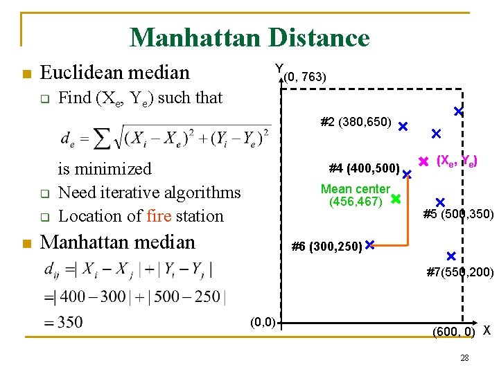
Manhattan Distance n Euclidean median q Y (0, 763) Find (Xe, Ye) such that #2 (380, 650) q q n is minimized Need iterative algorithms Location of fire station #4 (400, 500) Mean center (456, 467) Manhattan median (Xe, Ye) #5 (500, 350) #6 (300, 250) #7(550, 200) (0, 0) (600, 0) X 28

Summary n n n n What are spatial data? Mean center Weighted mean center Standard distance Weighted standard distance Euclidean median Calculate in GIS environment Manhattan median 29

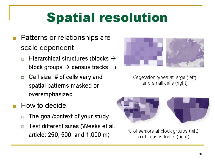
Spatial resolution n Patterns or relationships are scale dependent q q n Hierarchical structures (blocks block groups census tracks…) Cell size: # of cells vary and spatial patterns masked or overemphasized Vegetation types at large (left) and small cells (right) How to decide q q The goal/context of your study Test different sizes (Weeks et al. article: 250, 500, and 1, 000 m) % of seniors at block groups (left) and census tracts (right) 30

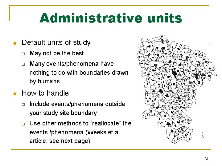
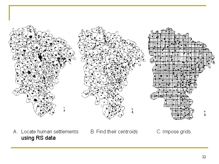
Administrative units n Default units of study q q n May not be the best Many events/phenomena have nothing to do with boundaries drawn by humans How to handle q q Include events/phenomena outside your study site boundary Use other methods to “reallocate” the events /phenomena (Weeks et al. article; see next page) 31

A. Locate human settlements B. Find their centroids C. Impose grids. using RS data 32

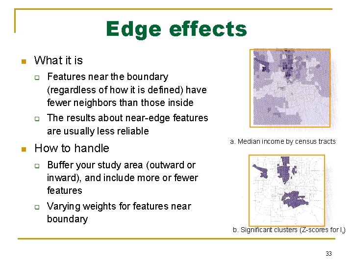
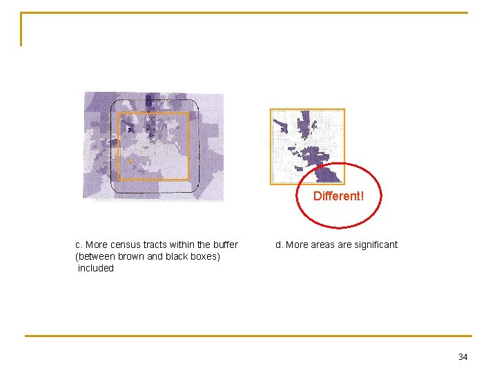
Edge effects n What it is q q n Features near the boundary (regardless of how it is defined) have fewer neighbors than those inside The results about near-edge features are usually less reliable How to handle q q a. Median income by census tracts Buffer your study area (outward or inward), and include more or fewer features Varying weights for features near boundary b. Significant clusters (Z-scores for Ii) 33

Different! c. More census tracts within the buffer (between brown and black boxes) included d. More areas are significant 34

Applying Spatial Statistics n n n Visualizing spatial data q Closely related to GIS q Other methods such as Histograms Exploring spatial data q Random spatial pattern or not q Tests about randomness Modeling spatial data q Correlation and 2 q Regression analysis 35