Dimension reduction and MD scaling Support Vector Machines


 and meta. PCA (in R) •")


 # effective dimension reduction library(dr) library(clustrd) install. packages(\"edr. Graphical. Tools\")")


 • cmdscale() (stats) • smacof. Sym() (smacof) • wcmdscale() (vegan)")
 cmdscale(d, k = 2, eig = FALSE, add = FALSE, x. ret =")
![Distances between Australian cities row. names(dist. au) <- dist. au[, 1] dist. au <-](https://slidetodoc.com/presentation_image_h2/91cdffdd9c727408e76a55102d035fc5/image-14.jpg "Distances between Australian cities row. names(dist. au) <- dist. au[, 1] dist. au <-")
")

 library(igraph) g <- graph. full(nrow(dist. au)) V(g)$label <-")

 • Lab 8 b_mds 1_2016. R • Lab 8 b_mds")
 classification, regression")
. svg")
 http: //en. wikipedia. org/wiki/File: Svm_max_sep_hyperplane_with_margin. png")


 using a function, i. e. a kernel Ø goal is")


 for certain and K,")


 • Classification SVM Type 1 (also known as CSVM classification)")


- Slides: 70
Dimension reduction and MD scaling, Support Vector Machines Peter Fox Data Analytics – 4600/6600 Week 9 a, March 29, 2016 1
Paid opportunity… 2 pm Fri • A small medical practice in Troy is considering opening a branch office in the Capital Region. They would like some GIS analysis to assist them in evaluating options for the location of the 2 nd office. Considerations would include demographics (with weighting by age), location of competitors (approximately 6), and drive-time analysis. They are open to considering other layers that might be suggested by the person(s) setting up the model. 2
Dimension reduction. . • Principle component analysis (PCA) and meta. PCA (in R) • Singular Value Decomposition • Feature selection, reduction • Built into a lot of clustering • Why? – Curse of dimensionality – or – some subset of the data should not be used as it adds noise • What is it? – Various methods to reach an optimal subset 3
Simple example 4
More dimensions 5
Feature selection • The goodness of a feature/feature subset is dependent on measures • Various measures – Information measures – Distance measures – Dependence measures – Consistency measures – Accuracy measures 6
On your own… library(EDR) # effective dimension reduction library(dr) library(clustrd) install. packages("edr. Graphical. Tools") library(edr. Graphical. Tools) demo(edr_ex 1) demo(edr_ex 2) demo(edr_ex 3) demo(edr_ex 4) 7
Some examples • • Lab 8 b_dr 1_2016. R Lab 8 b_dr 2_2016. R Lab 8 b_dr 3_2016. R Lab 8 b_dr 4_2016. R 8
Multidimensional Scaling • Visual representation ~ 2 -D plot - patterns of proximity in a lower dimensional space • "Similar" to PCA/DR but uses dissimilarity as input > dissimilarity matrix – An MDS algorithm aims to place each object in Ndimensional space such that the between-object distances are preserved as well as possible. – Each object is then assigned coordinates in each of the N dimensions. – The number of dimensions of an MDS plot N can exceed 2 and is specified a priori. – Choosing N=2 optimizes the object locations for a twodimensional scatterplot 9
Four types of MDS • Classical multidimensional scaling – Also known as Principal Coordinates Analysis, Torgerson Scaling or Torgerson–Gower scaling. Takes an input matrix giving dissimilarities between pairs of items and outputs a coordinate matrix whose configuration minimizes a loss function called strain. • Metric multidimensional scaling – A superset of classical MDS that generalizes the optimization procedure to a variety of loss functions and input matrices of known distances with weights and so on. A useful loss function in this context is called stress, which is often minimized using a procedure called stress majorization. 10
Four types of MDS ctd • Non-metric multidimensional scaling – In contrast to metric MDS, non-metric MDS finds both a non-parametric monotonic relationship between the dissimilarities in the item-item matrix and the Euclidean distances between items, and the location of each item in the low-dimensional space. The relationship is typically found using isotonic regression. • Generalized multidimensional scaling – An extension of metric multidimensional scaling, in which the target space is an arbitrary smooth non-Euclidean space. In cases where the dissimilarities are distances on a surface and the target space is another surface, GMDS allows finding the minimum-distortion embedding of one surface into another. 11
In R function (library) • cmdscale() (stats) • smacof. Sym() (smacof) • wcmdscale() (vegan) • pco() (ecodist) • pco() (labdsv) • pcoa() (ape) • Only stats is loaded by default, and the rest are not installed by default 12
cmdscale() cmdscale(d, k = 2, eig = FALSE, add = FALSE, x. ret = FALSE) d - a distance structure such as that returned by dist or a full symmetric matrix containing the dissimilarities. k - the maximum dimension of the space which the data are to be represented in; must be in {1, 2, …, n-1}. eig - indicates whether eigenvalues should be returned. add - logical indicating if an additive constant c* should be computed, and added to the non-diagonal dissimilarities such that the modified dissimilarities are Euclidean. x. ret - indicates whether the doubly centred symmetric distance matrix should be returned. 13
Distances between Australian cities row. names(dist. au) <- dist. au[, 1] dist. au <- dist. au[, -1] dist. au ## A AS B D H M P S ## A 0 1328 1600 2616 1161 653 2130 1161 ## AS 1328 0 1962 1289 2463 1889 1991 2026 ## B 1600 1962 0 2846 1788 1374 3604 732 ## D 2616 1289 2846 0 3734 3146 2652 3146 ## H 1161 2463 1788 3734 0 598 3008 1057 ## M 653 1889 1374 3146 598 0 2720 713 ## P 2130 1991 3604 2652 3008 2720 0 3288 ## S 1161 2026 732 3146 1057 713 3288 0 14
Distances between Australian cities fit <- cmdscale(dist. au, eig = TRUE, k = 2) x <- fit$points[, 1] y <- fit$points[, 2] plot(x, y, pch = 19, xlim = range(x) + c(0, 600)) city. names <- c("Adelaide", "Alice Springs", "Brisbane", "Darwin", "Hobart", "Melbourne", "Perth", "Sydney") text(x, y, pos = 4, labels = city. names) 15
16
R – many ways (of course) library(igraph) g <- graph. full(nrow(dist. au)) V(g)$label <- city. names layout <- layout. mds(g, dist = as. matrix(dist. au)) plot(g, layout = layout, vertex. size = 3) 17
18
On your own (Friday) • Lab 8 b_mds 1_2016. R • Lab 8 b_mds 2_2016. R • Lab 8 b_mds 3_2016. R • http: //www. statmethods. net/advstats/mds. htm l • http: //gastonsanchez. com/blog/howto/2013/01/23/MDS-in-R. html 19
Support Vector Machine • Conceptual theory, formulae… • SVM - general (nonlinear) classification, regression and outlier detection with an intuitive model representation • Hyperplanes separate the classification spaces (can be multi-dimensional) • Kernel functions can play a key role 20
Schematically 21 http: //en. wikipedia. org/wiki/File: Svm_separating_hyperplanes_(SVG). svg
Schematically Support Vectors 22 b=bias term, b=0 (unbiased) http: //en. wikipedia. org/wiki/File: Svm_max_sep_hyperplane_with_margin. png
Construction • Construct an optimization objective function that is inherently subject to some constraints – Like minimizing least square error (quadratic) • Most important: the classifier gets the points right by “at least” the margin • Support Vectors can then be defined as those points in the dataset that have "non zero” Lagrange multipliers*. – make a classification on a new point by using only the support vectors – why? 23
Support vectors • Support the “plane” 24
What about the “machine” part • Ignore it – somewhat leftover from the “machine learning” era – It is trained and then – Classifies 25
No clear separation = no hyperplane? Soft-margins… Non-linearity or transformation 26
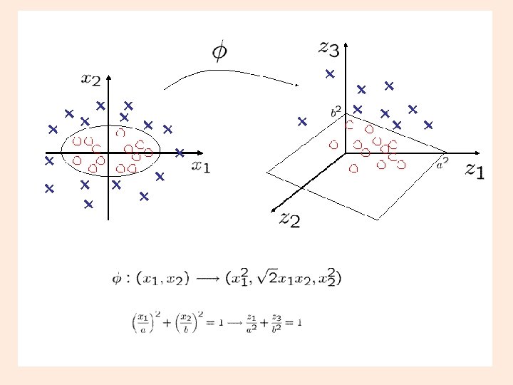
Feature space Mapping (transformation) using a function, i. e. a kernel Ø goal is – linear separability 27
Kernels or “non-linearity”… http: //www. statsoft. com/Textbook/Support-Vector-Machines the kernel function, represents a dot product of input data points mapped into the higher dimensional feature space by transformation phi + note presence of “gamma” parameter 28
Best Linear Separator: Supporting Plane Method Maximize distance Between two paral supporting planes Distance = “Margin” =
Soft Margin SVM Just add non-negative error vector z.
Method 2: Find Closest Points in Convex Hulls d c
Plane Bisects Closest Points d c
Find using quadratic program Many existing and new QP solvers.
Dual of Closest Points Method is Support Plane Method Solution only depends on support vectors:
One bad example? Convex Hulls Intersect! Same argument won’t work.
Don’t trust a single point! Each point must depend on at least two actual data points.
Depend on >= two points Each point must depend on at least two actual data points.
Depend on >= two points Each point must depend on at least two actual data points.
Depend on >= two points Each point must depend on at least two actual data points.
Depend on >= two points Each point must depend on at least two actual data points.
Final Reduced/Robust Set Each point must depend on at least two actual data points Called Reduced Convex Hull
Reduced Convex Hulls Don’t Intersect Reduce by adding upper bound D
Find Closest Points Then Bisect No change except for D. D determines number of Support Vectors.
Dual of Closest Points Method is Soft Margin Method Solution only depends on support vectors:
What will linear SVM do?
Linear SVM Fails
High Dimensional Mapping trick http: //www. slideshare. net/ankitksh arma/svm-37753690
Nonlinear Classification: Map to higher dimensional space IDEA: Map each point to higher dimensional feature space and construct linear discriminant in the higher dimensional space. Dual SVM becomes:
Kernel Calculates Inner Product
Final Classification via Kernels The Dual SVM becomes:
Generalized Inner Product By Hilbert-Schmidt Kernels (Courant and Hilbert 1953) for certain and K, e. g. Also kernels for nonvector data like strings, histograms, dna, …
Final SVM Algorithm • Solve Dual SVM QP • Recover primal variable b • Classify new x Solution only depends on support vectors:
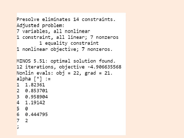
SVM AMPL DUAL MODEL
S 5: Recal linear solution
RBF results on Sample Data
Have to pick parameters Effect of C
Effect of RBF parameter
General Kernel methodology • • • Pick a learning task Start with linear function and data Define loss function Define regularization Formulate optimization problem in dual space/inner product space • Construct an appropriate kernel • Solve problem in dual space
kernlab, svmpath and kla. R • http: //escience. rpi. edu/data/DA/v 15 i 09. pdf Karatzoglou et al. 2006 • Work through the examples – Familiar datasets and samples procedures from 4 libraries (these are the most used) – kernlab – e 1071 – svmpath – kla. R 61
Application of SVM • Classification, outlier, regression… • Can produce labels or probabilities (and when used with tree partitioning can produce decision values) • Different minimizations functions subject to different constraints (Lagrange multipliers) See Karatzoglou et al. 2006 • Observe the effect of changing the C parameter and the kernel 62
Types of SVM (names) • Classification SVM Type 1 (also known as CSVM classification) • Classification SVM Type 2 (also known as nu. SVM classification) • Regression SVM Type 1 (also known as epsilon-SVM regression) • Regression SVM Type 2 (also known as nu. SVM regression) 63
More kernels 64 Karatzoglou et al. 2006
Timing 65 Karatzoglou et al. 2006
Library capabilities Karatzoglou et al. 2006 66
Extensions • Many Inference Tasks – – – – Regression One-class Classification, novelty detection Ranking Clustering Multi-Task Learning Kernels Cannonical Correlation Analysis Principal Component Analysis
Algorithms Types: • General Purpose solvers – CPLEX by ILOG – Matlab optimization toolkit • Special purpose solvers exploit structure of the problem – Best linear SVM take time linear in the number of training data points. – Best kernel SVM solvers take time quadratic in the number of training data points. • Good news since convex, algorithm doesn’t really matter as long as solvable.
Hallelujah! • Generalization theory and practice meet • General methodology for many types of inference problems • Same Program + New Kernel = New method • No problems with local minima • Few model parameters. Avoids overfitting • Robust optimization methods. • Applicable to non-vector problems. • Easy to use and tune • Successful Applications BUT…
Catches • Will SVMs beat my best hand-tuned method Z on problem X? • Do SVMs scale to massive datasets? • How to chose C and Kernel? • How to transform data? • How to incorporate domain knowledge? • How to interpret results? • Are linear methods enough?