Support Vector Machines Jeff Wu 1 1 Support

Support Vector Machines Jeff Wu 1

1 Support Vector Machines: history SVMs close to their current form were first introduced in COLT-92 by Boser, Guyon & Vapnik. Became rather popular since then. But the history of SVMs goes way back. In 1936, R. A. Fisher suggested the first algorithm for pattern recognition (Fisher 1936), called “discriminant analysis”. Aronszajn (1950) introduced the ‘Theory of Reproducing Kernels’. Vapnik and Lerner (1963) introduced the Generalized Portrait algorithm (the algorithm implemented by support vector machines is a nonlinear generalization of the Generalized Portrait algorithm). Vapnik and Chervonenkis (1964) further develop the Generalized Portrait algorithm. Cover (1965) discussed large margin hyperplanes in the input space and also sparseness. 2

1 Support Vector Machines: history The field of ‘statistical learning theory’ began with Vapnik and Chervonenkis (1974) (in Russian). SVMs can be said to have started when statistical learning theory was developed further with Vapnik (1979) (in Russian). Vapnik (1982) wrote an English translation of his 1979 book. In 1995 the soft margin classifier was introduced by Cortes and Vapnik (1995); in the same year the algorithm was extended to the case of regression by Vapnik (1995) in The Nature of Statistical Learning Theory. The papers by Bartlett (1998) and Shawe-Taylor, et al. (1998) gave the first rigorous statistical bounds on the generalisation of hard margin SVMs. Shawe-Taylor and Cristianini (2000) gave statistical bounds on the generalisation of soft margin algorithms and for the regression case. 3

2 Why SVMs Empirically good performance: successful applications in many fields. (bioinformatics, text, image recognition, . . . ) For the pattern recognition case, SVMs have been used for isolated handwritten digit recognition (Cortes and Vapnik, 1995; Scholkopf, Burges and Vapnik, 1996; Burges and Scholkopf, 1997), object recognition (Blanz et al. , 1996), speaker identification (Schmidt, 1996), charmed quark detection 1, face detection in images (Osuna, Freund and Girosi, 1997 a), and text categorization. (Joachims, 1997) For the regression estimation case, SVMs have been compared on benchmark time series prediction tests (Muller et al. , 1997; Mukherjee, Osuna and Girosi, 1997), the Boston housing problem (Drucker et al. , 2 1997), and (on artificial data) on the PET operator inversion problem. (Vapnik, Golowich and Smola, 1996) In most of these cases, SVM generalization performance (i. e. error rates on test sets) either matches or is significantly better than that of competing methods. 4

Today’s Agenda VC dimension Linear SVMs (with both separable and non-separable cases) Non-linear SVMs (Kernel trick) 5

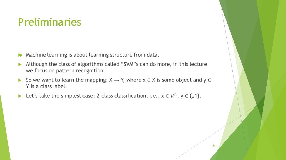
Preliminaries 6

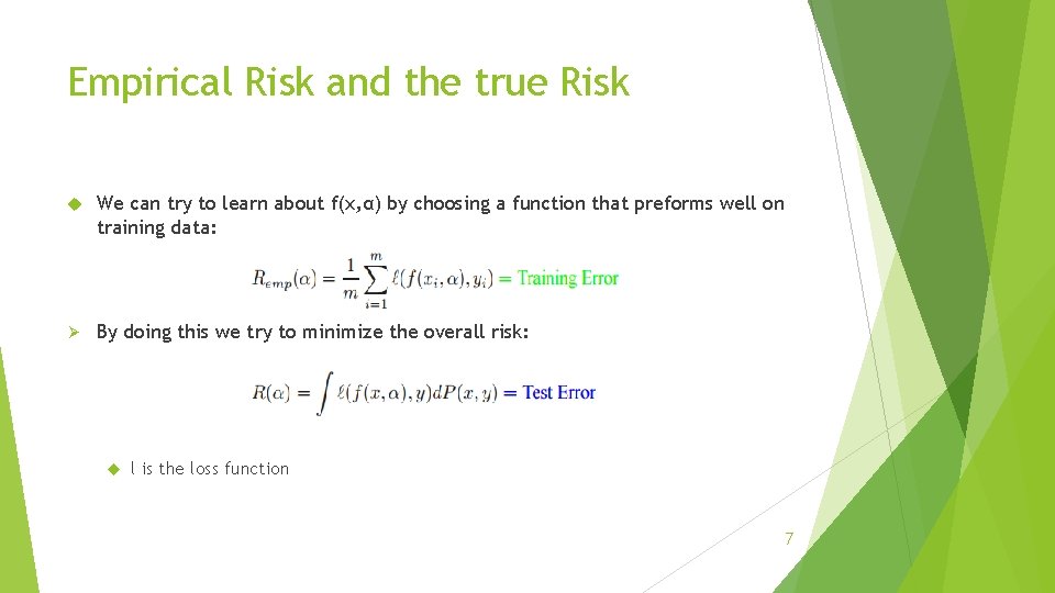
Empirical Risk and the true Risk We can try to learn about f(x, α) by choosing a function that preforms well on training data: Ø By doing this we try to minimize the overall risk: l is the loss function 7

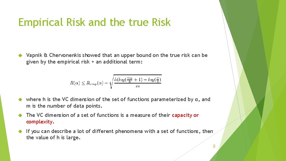
Empirical Risk and the true Risk Vapnik & Chervonenkis showed that an upper bound on the true risk can be given by the empirical risk + an additional term: where h is the VC dimension of the set of functions parameterized by α, and m is the number of data points. The VC dimension of a set of functions is a measure of their capacity or complexity. If you can describe a lot of different phenomena with a set of functions, then the value of h is large. 8

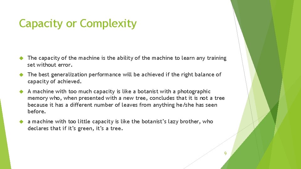
Capacity or Complexity The capacity of the machine is the ability of the machine to learn any training set without error. The best generalization performance will be achieved if the right balance of capacity of achieved. A machine with too much capacity is like a botanist with a photographic memory who, when presented with a new tree, concludes that it is not a tree because it has a different number of leaves from anything he/she has seen before. a machine with too little capacity is like the botanist’s lazy brother, who declares that if it’s green, it’s a tree. 9

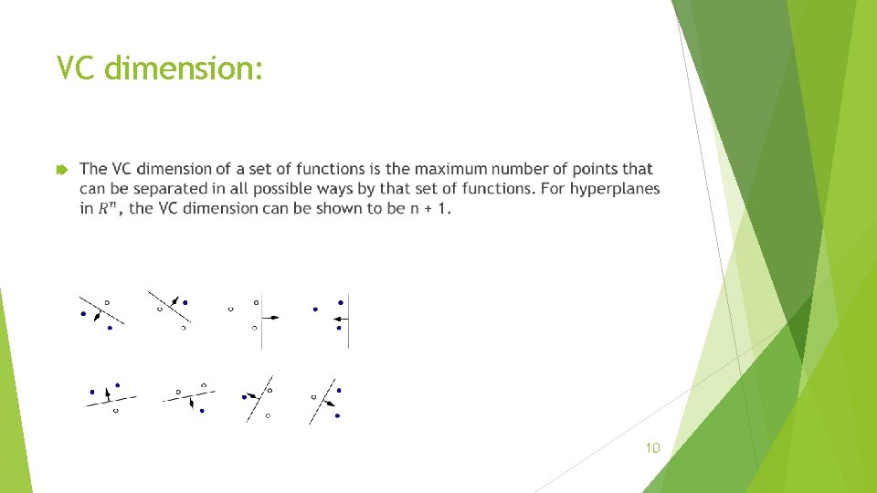
VC dimension: 10

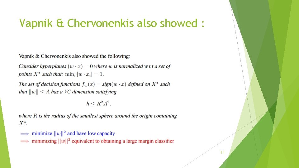
Vapnik & Chervonenkis also showed : 11

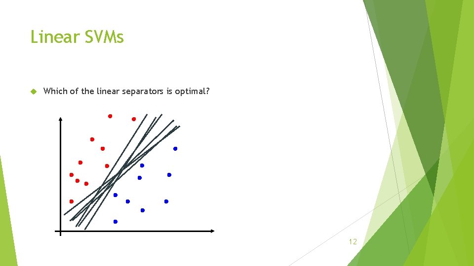
Linear SVMs Which of the linear separators is optimal? 12

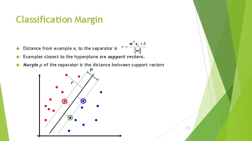
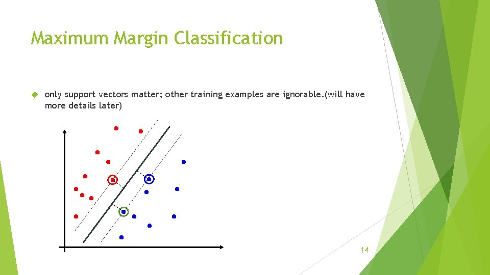
Classification Margin Distance from example xi to the separator is Examples closest to the hyperplane are support vectors. Margin ρ of the separator is the distance between support vectors ρ r 13

Maximum Margin Classification only support vectors matter; other training examples are ignorable. (will have more details later) 14

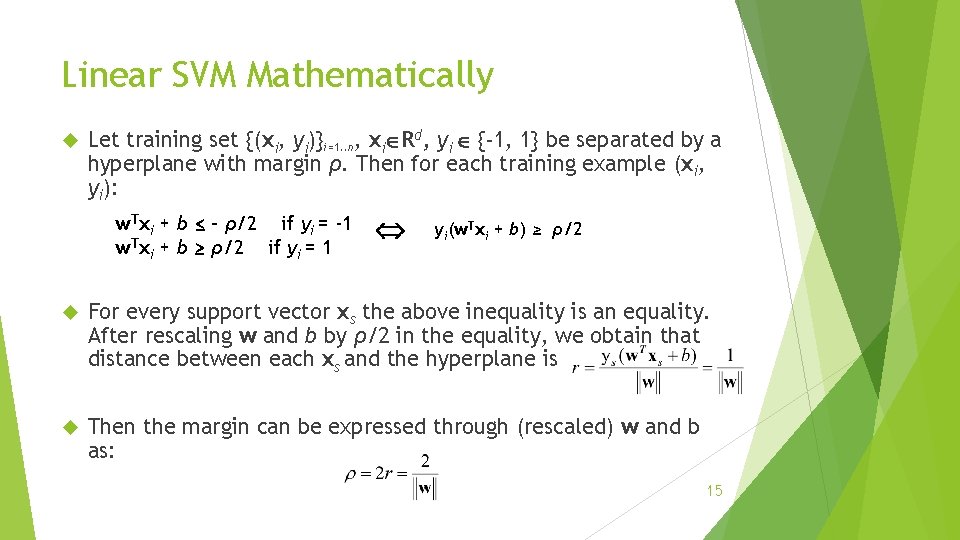
Linear SVM Mathematically Let training set {(xi, yi)}i=1. . n, xi Rd, yi {-1, 1} be separated by a hyperplane with margin ρ. Then for each training example (xi, yi): w. Txi + b ≤ - ρ/2 if yi = -1 w. Txi + b ≥ ρ/2 if yi = 1 yi(w. Txi + b) ≥ ρ/2 For every support vector xs the above inequality is an equality. After rescaling w and b by ρ/2 in the equality, we obtain that distance between each xs and the hyperplane is Then the margin can be expressed through (rescaled) w and b as: 15

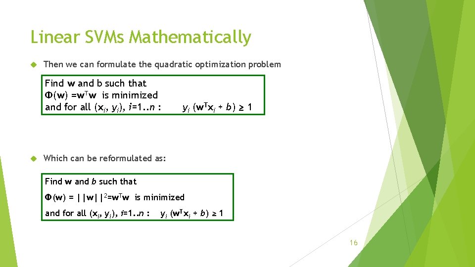
Linear SVMs Mathematically Then we can formulate the quadratic optimization problem Find w and b such that Φ(w) =w. Tw is minimized and for all (xi, yi), i=1. . n : yi (w. Txi + b) ≥ 1 Which can be reformulated as: Find w and b such that Φ(w) = ||w||2=w. Tw is minimized and for all (xi, yi), i=1. . n : yi (w. Txi + b) ≥ 1 16

Solving the Optimization Problem Quadratic optimization problems are a well-known class of mathematical programming problems for which several (non-trivial) algorithms are available. The solution involves constructing a dual problem. 17

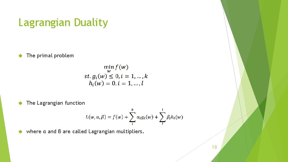
Lagrangian Duality The primal problem The Lagrangian function where α and β are called Lagrangian multipliers. 18

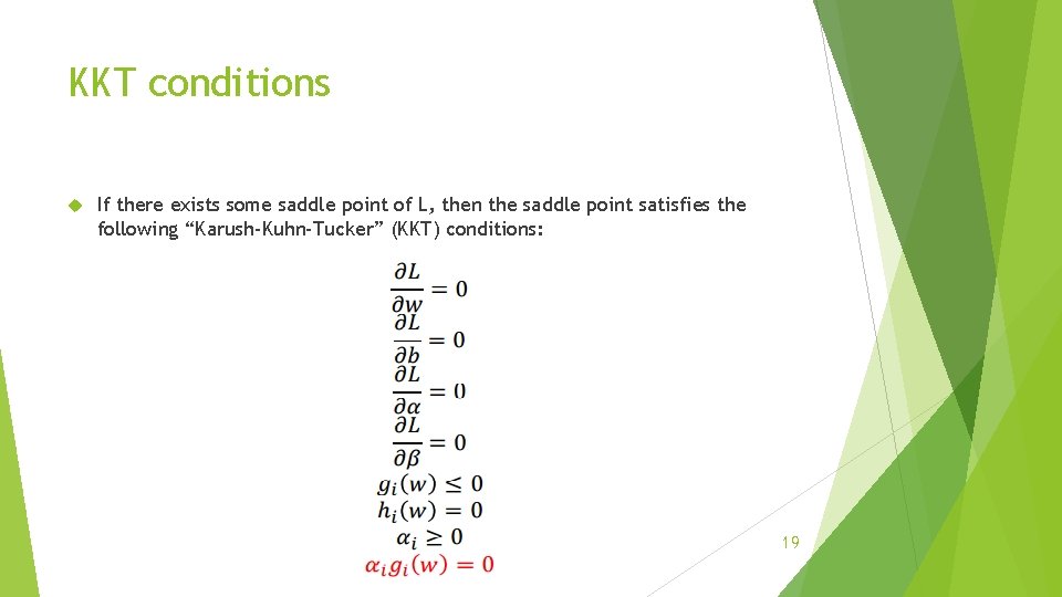
KKT conditions If there exists some saddle point of L, then the saddle point satisfies the following “Karush-Kuhn-Tucker” (KKT) conditions: 19

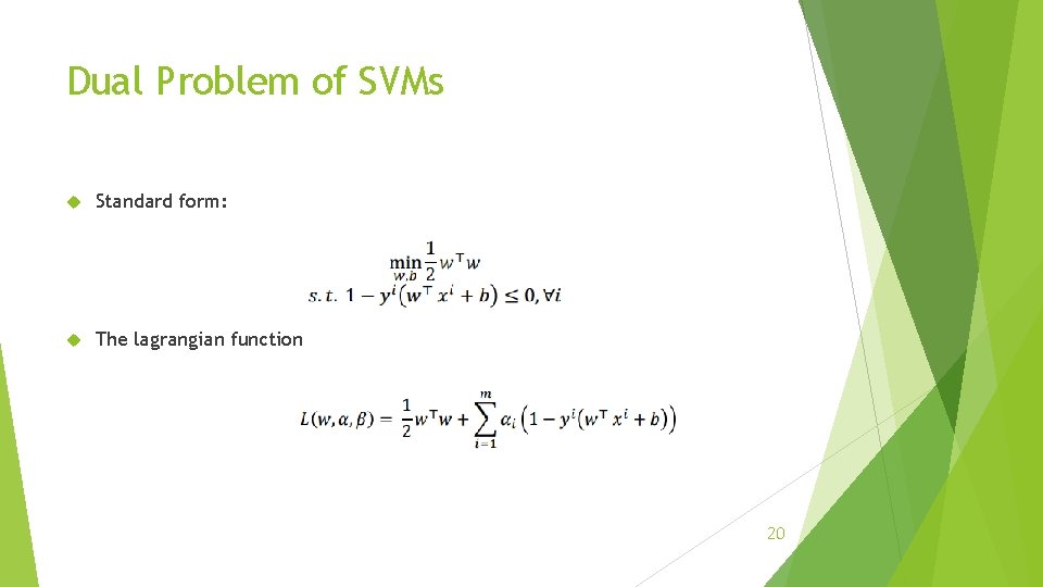
Dual Problem of SVMs Standard form: The lagrangian function 20

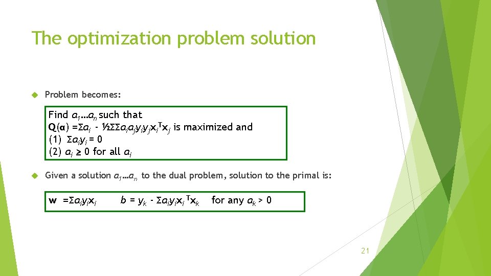
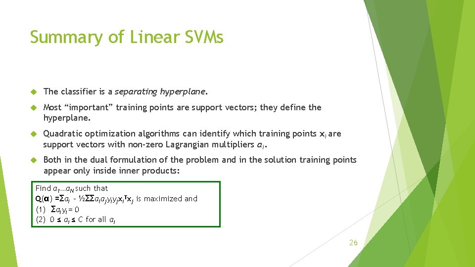
The optimization problem solution Problem becomes: Find α 1…αn such that Q(α) =Σαi - ½ΣΣαiαjyiyjxi. Txj is maximized and (1) Σαiyi = 0 (2) αi ≥ 0 for all αi Given a solution α 1…αn to the dual problem, solution to the primal is: w =Σαiyixi b = yk - Σαiyixi Txk for any αk > 0 21

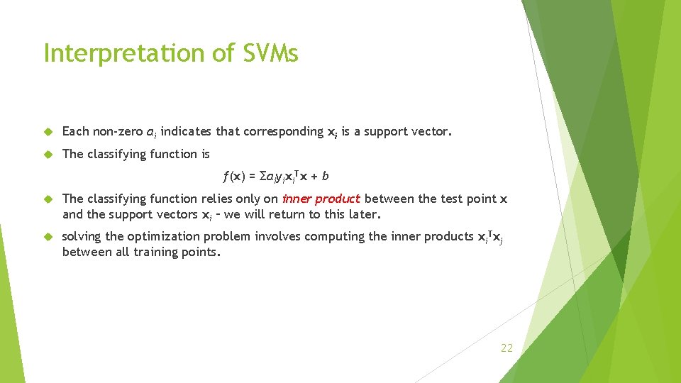
Interpretation of SVMs Each non-zero αi indicates that corresponding xi is a support vector. The classifying function is f(x) = Σαiyixi. Tx + b The classifying function relies only on inner product between the test point x and the support vectors xi – we will return to this later. solving the optimization problem involves computing the inner products xi. Txj between all training points. 22

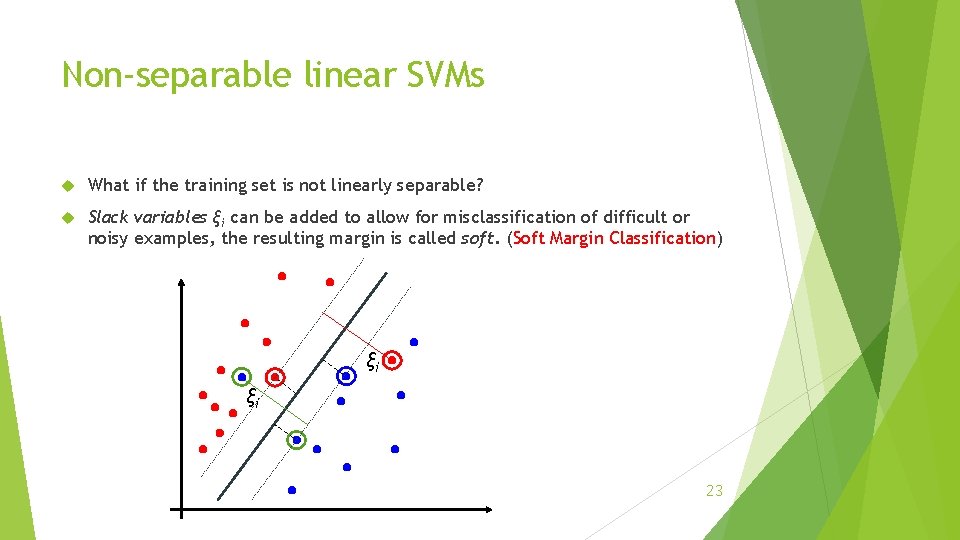
Non-separable linear SVMs What if the training set is not linearly separable? Slack variables ξi can be added to allow for misclassification of difficult or noisy examples, the resulting margin is called soft. (Soft Margin Classification) ξi ξi 23

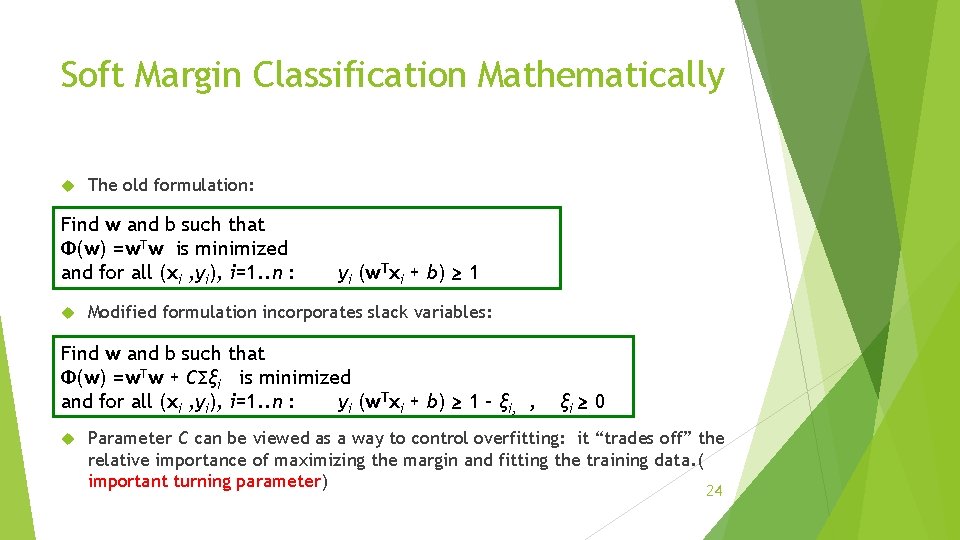
Soft Margin Classification Mathematically The old formulation: Find w and b such that Φ(w) =w. Tw is minimized and for all (xi , yi), i=1. . n : yi (w. Txi + b) ≥ 1 Modified formulation incorporates slack variables: Find w and b such that Φ(w) =w. Tw + CΣξi is minimized and for all (xi , yi), i=1. . n : yi (w. Txi + b) ≥ 1 – ξi, , ξi ≥ 0 Parameter C can be viewed as a way to control overfitting: it “trades off” the relative importance of maximizing the margin and fitting the training data. ( important turning parameter) 24

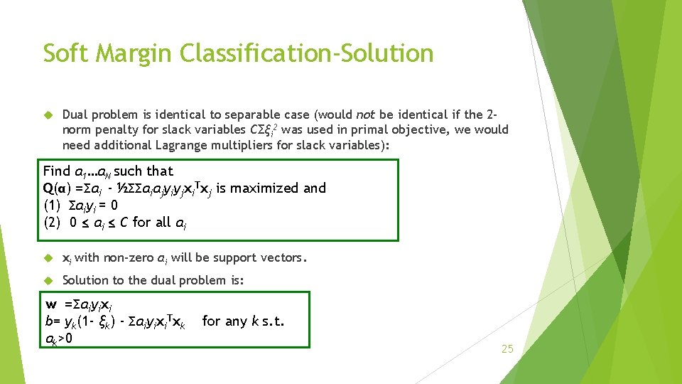
Soft Margin Classification-Solution Dual problem is identical to separable case (would not be identical if the 2 norm penalty for slack variables CΣξi 2 was used in primal objective, we would need additional Lagrange multipliers for slack variables): Find α 1…αN such that Q(α) =Σαi - ½ΣΣαiαjyiyjxi. Txj is maximized and (1) Σαiyi = 0 (2) 0 ≤ αi ≤ C for all αi xi with non-zero αi will be support vectors. Solution to the dual problem is: w =Σαiyixi b= yk(1 - ξk) - Σαiyixi. Txk αk>0 for any k s. t. 25

Summary of Linear SVMs The classifier is a separating hyperplane. Most “important” training points are support vectors; they define the hyperplane. Quadratic optimization algorithms can identify which training points xi are support vectors with non-zero Lagrangian multipliers αi. Both in the dual formulation of the problem and in the solution training points appear only inside inner products: Find α 1…αN such that Q(α) =Σαi - ½ΣΣαiαjyiyjxi. Txj is maximized and (1) Σαiyi = 0 (2) 0 ≤ αi ≤ C for all αi 26

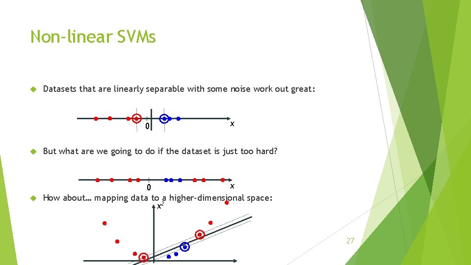
Non-linear SVMs Datasets that are linearly separable with some noise work out great: 0 x But what are we going to do if the dataset is just too hard? x 0 How about… mapping data to a higher-dimensional space: x 2 27

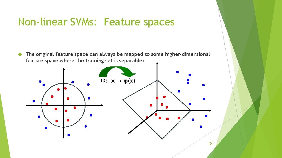
Non-linear SVMs: Feature spaces The original feature space can always be mapped to some higher-dimensional feature space where the training set is separable: Φ: x → φ(x) 28

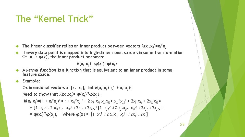
The “Kernel Trick” The linear classifier relies on inner product between vectors K(xi, xj)=xi. Txj If every data point is mapped into high-dimensional space via some transformation Φ: x → φ(x), the inner product becomes: K(xi, xj)= φ(xi) Tφ(xj) A kernel function is a function that is equivalent to an inner product in some feature space. Example: 2 -dimensional vectors x=[x 1 x 2]; let K(xi, xj)=(1 + xi. Txj)2, Need to show that K(xi, xj)= φ(xi) Tφ(xj): K(xi, xj)=(1 + xi. Txj)2, = 1+ xi 12 xj 12 + 2 xi 1 xj 1 xi 2 xj 2+ xi 22 xj 22 + 2 xi 1 xj 1 + 2 xi 2 xj 2= = [1 xi 12 √ 2 xi 1 xi 22 √ 2 xi 1 √ 2 xi 2]T [1 xj 12 √ 2 xj 1 xj 22 √ 2 xj 1 √ 2 xj 2] = = φ(xi) Tφ(xj), where φ(x) = [1 x 12 √ 2 x 1 x 2 x 22 √ 2 x 1 √ 2 x 2] 29

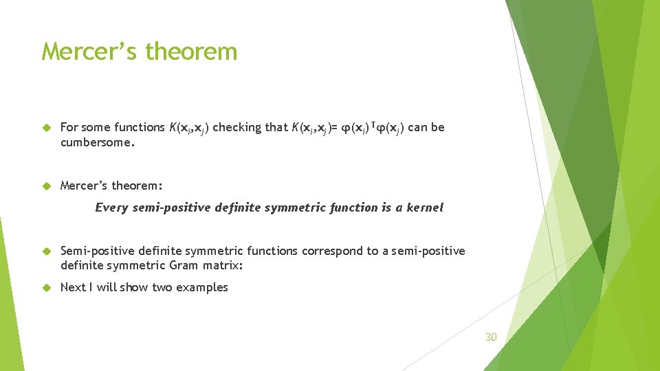
Mercer’s theorem For some functions K(xi, xj) checking that K(xi, xj)= φ(xi) Tφ(xj) can be cumbersome. Mercer’s theorem: Every semi-positive definite symmetric function is a kernel Semi-positive definite symmetric functions correspond to a semi-positive definite symmetric Gram matrix: Next I will show two examples 30

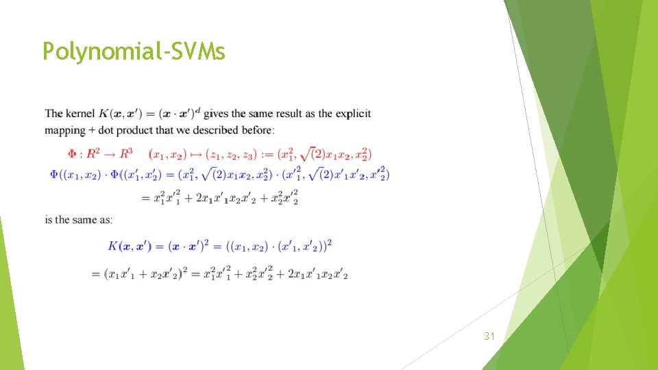
Polynomial-SVMs 31

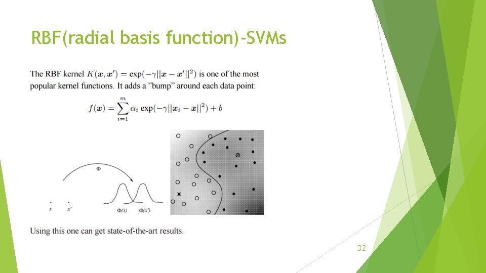
RBF(radial basis function)-SVMs 32

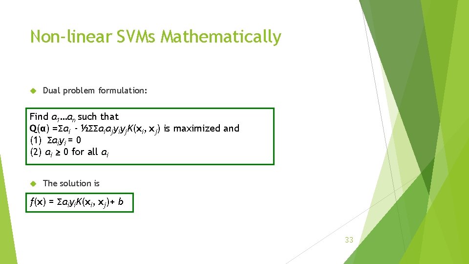
Non-linear SVMs Mathematically Dual problem formulation: Find α 1…αn such that Q(α) =Σαi - ½ΣΣαiαjyiyj. K(xi, xj) is maximized and (1) Σαiyi = 0 (2) αi ≥ 0 for all αi The solution is f(x) = Σαiyi. K(xi, xj)+ b 33

SVMs: more results There is much more in the field of SVMs/ kernel machines than we could cover here, including: Regression, clustering, semi-supervised learning and other domains. Lots of other kernels, e. g. string kernels to handle text. Lots of research in modifications, e. g. to improve generalization ability, or tailoring to a particular task. Lots of research in speeding up training. 34

Readings: Element of statistical learning(2 nd edition) by Jerome H. Friedman, Robert Tibshirani, and Trevor Hastie Chapter 6, 12 Pattern Recognition and Machine Learning by Christopher Bishop Chapter 6, 7 A tutorial by Christopher Burges: http: //research. microsoft. com/en-us/um/people/cburges/papers/svmtutorial. pdf http: //www. kernel-machines. org/ http: //www. svms. org/ 35