10 0 Latent Semantic Analysis for Linguistic Processing

10. 0 Latent Semantic Analysis for Linguistic Processing References: 1. “Exploiting Latent Semantic Information in Statistical Language Modeling”, Proceedings of the IEEE, Aug 2000 2. “Latent Semantic Mapping”, IEEE Signal Processing Magazine, Sept. 2005, Special Issue on Speech Technology in Human-Machine Communication 3. “Golub & Van Loan, “ Matrix Computations ”, 1989 4. “Probabilistic Latent Semantic Indexing”, ACM Special Interest Group on Information Retrieval (ACM SIGIR), 1999 5. “Probabilistic Latent Semantic Indexing”, Proc. of Uncertainty in Artificial Intelligence, 1999 6. “Spoken Document Understanding and Organization”, IEEE Signal Processing Magazine, Sept. 2005, Special Issue on Speech Technology in Human-Machine Communication

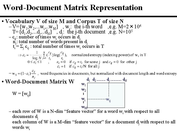
Word-Document Matrix Representation • Vocabulary V of size M and Corpus T of size N – V={w 1, w 2, . . . wi, . . w. M} , wi: the i-th word , e. g. M=2× 104 T={d 1, d 2, . . . dj, . . d. N} , dj: the j-th document , e. g. N=105 – cij: number of times wi occurs in dj nj: total number of words present in dj ti = Σj cij : total number of times wi occurs in T – • Word-Document Matrix W W = [wij] w 1 w 2 d 1 d 2. . . . dj. . d. N wi w. M wij – each row of W is a N-dim “feature vector” for a word wi with respect to all documents dj each column of W is a M-dim “feature vector” for a document dj with respect to all words wi

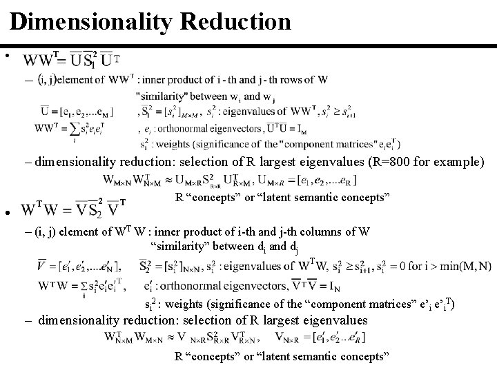
Dimensionality Reduction • T 2 – – dimensionality reduction: selection of R largest eigenvalues (R=800 for example) • T 2 T R “concepts” or “latent semantic concepts” – (i, j) element of WT W : inner product of i-th and j-th columns of W “similarity” between di and dj T si 2 : weights (significance of the “component matrices” e’i. T) – dimensionality reduction: selection of R largest eigenvalues R “concepts” or “latent semantic concepts”

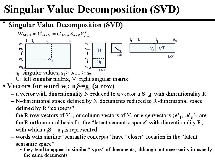
Singular Value Decomposition (SVD) • Singular Value Decomposition (SVD) w 1 w 2 wi w. M d 1 d 2. . . . dj. wij . . d. N w 1 w 2 = wi w. M d 1 s 1 U s. R R×R ui d 2. . . . dj. . d. N T vj VT R×N M×R – si: singular values, s 1≥ s 2. . ≥ s. R U: left singular matrix, V: right singular matrix • Vectors for word wi: ui. S=ui (a row) – a vector with dimentionality N reduced to a vector ui. S=ui with dimentionality R – N-dimentional space defined by N documents reduced to R-dimentional space defined by R “concepts” – the R row vectors of VT, or column vectors of V, or eigenvectors {e’ 1, . . e’R}, are the R orthonormal basis for the “latent semantic space” with dimentionality R, with which ui. S = u i is represented – words with similar “semantic concepts” have “closer” location in the “latent semantic space” • they tend to appear in similar “types” of documents, although not necessarily in exactly the same documents

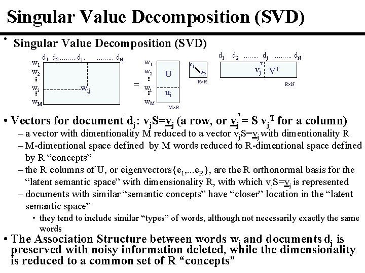
Singular Value Decomposition (SVD) • Singular Value Decomposition (SVD) w 1 w 2 wi w. M d 1 d 2. . . . dj. wij . . d. N w 1 w 2 = wi w. M d 1 s 1 U d 2. . . . dj. . d. N T vj VT s. R R×N ui M×R T • Vectors for document dj: vj. S=vj (a row, or vj = S vj. T for a column) – a vector with dimentionality M reduced to a vector vj. S=vj with dimentionality R – M-dimentional space defined by M words reduced to R-dimentional space defined by R “concepts” – the R columns of U, or eigenvectors{e 1, . . . e. R}, are the R orthonormal basis for the “latent semantic space” with dimensionality R, with which vj. S=vj is represented – documents with similar “semantic concepts” have “closer” location in the “latent semantic space” • they tend to include similar “types” of words, although not necessarily exactly the same words • The Association Structure between words wi and documents dj is preserved with noisy information deleted, while the dimensionality is reduced to a common set of R “concepts”

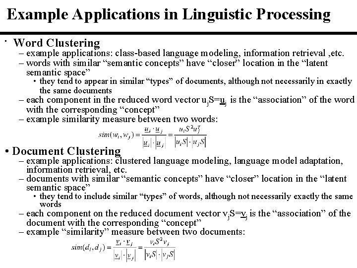
Example Applications in Linguistic Processing • Word Clustering – example applications: class-based language modeling, information retrieval , etc. – words with similar “semantic concepts” have “closer” location in the “latent semantic space” • they tend to appear in similar “types” of documents, although not necessarily in exactly the same documents – each component in the reduced word vector uj. S=uj is the “association” of the word with the corresponding “concept” – example similarity measure between two words: 2 • Document Clustering – example applications: clustered language modeling, language model adaptation, information retrieval, etc. – documents with similar “semantic concepts” have “closer” location in the “latent semantic space” • they tend to include similar “types” of words, although not necessarily exactly the same words – each component on the reduced document vector vj. S=vj is the “association” of the document with the corresponding “concept” – example “similarity” measure between two documents: 2

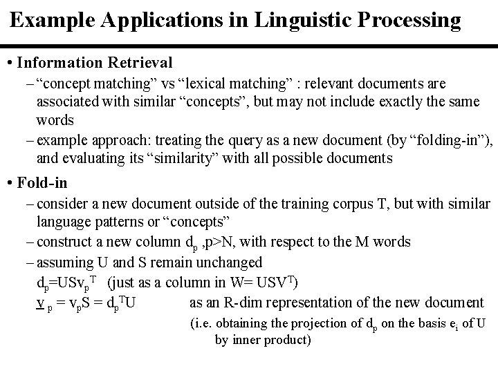
Example Applications in Linguistic Processing • Information Retrieval – “concept matching” vs “lexical matching” : relevant documents are associated with similar “concepts”, but may not include exactly the same words – example approach: treating the query as a new document (by “folding-in”), and evaluating its “similarity” with all possible documents • Fold-in – consider a new document outside of the training corpus T, but with similar language patterns or “concepts” – construct a new column dp , p>N, with respect to the M words – assuming U and S remain unchanged dp=USvp. T (just as a column in W= USVT) v p = vp. S = dp. TU as an R-dim representation of the new document (i. e. obtaining the projection of dp on the basis ei of U by inner product)

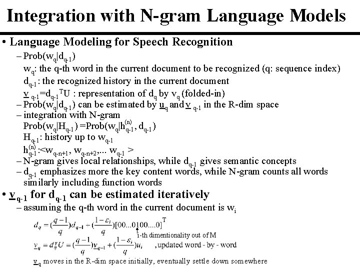
Integration with N-gram Language Models • Language Modeling for Speech Recognition – Prob(wq|dq-1) wq: the q-th word in the current document to be recognized (q: sequence index) dq-1: the recognized history in the current document v q-1=dq-1 TU : representation of dq by vq (folded-in) – Prob(wq|dq-1) can be estimated by uq and v q-1 in the R-dim space – integration with N-gram (n) Prob(wq|Hq-1) =Prob(wq|hq-1, dq-1) Hq-1: history up to wq-1 (n) hq-1 : <wq-n+1, wq-n+2, . . . wq-1 > – N-gram gives local relationships, while dq-1 gives semantic concepts – dq-1 emphasizes more the key content words, while N-gram counts all words similarly including function words • v q-1 for dq-1 can be estimated iteratively – assuming the q-th word in the current document is wi T i-th dimentionality out of M v q moves in the R-dim space initially, eventually settle down somewhere

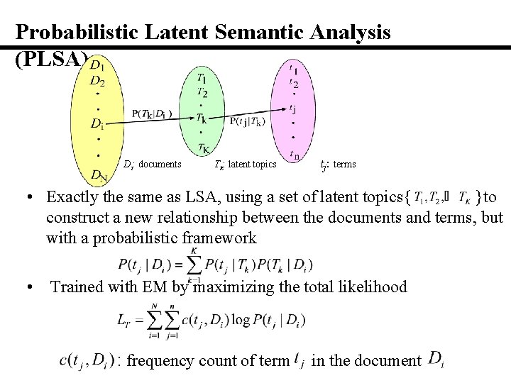
Probabilistic Latent Semantic Analysis (PLSA) Di: documents Tk: latent topics tj: terms • Exactly the same as LSA, using a set of latent topics{ }to construct a new relationship between the documents and terms, but with a probabilistic framework • Trained with EM by maximizing the total likelihood : frequency count of term in the document