Chapter 3 Vector Spaces n n n n
![§ Notes: If rank([A|b])=rank(A) (Thm 3. 18) 3. 18 Then the system Ax=b is § Notes: If rank([A|b])=rank(A) (Thm 3. 18) 3. 18 Then the system Ax=b is](https://slidetodoc.com/presentation_image_h/e2bff8f0f6d568359f3121bfb16656c4/image-74.jpg)
![n Transition matrix from B' to B: If [v]B is the coordinate matrix of n Transition matrix from B' to B: If [v]B is the coordinate matrix of](https://slidetodoc.com/presentation_image_h/e2bff8f0f6d568359f3121bfb16656c4/image-82.jpg)
- Slides: 89

Chapter 3 Vector Spaces n n n n 3. 1 Vectors in Rn 3. 2 Vector Spaces 3. 3 Subspaces of Vector Spaces 3. 4 Spanning Sets and Linear Independence 3. 5 Basis and Dimension 3. 6 Rank of a Matrix and Systems of Linear Equations 3. 7 Coordinates and Change of Basis The idea of vectors dates back to the early 1800’s, but the generality of the concept waited until Peano’s work in 1888. It took many years to understand the importance and extent of the ideas involved. The underlying idea can be used to describe the forces and accelerations in Newtonian mechanics and the potential functions of electromagnetism and the mechanics electromagnetism states of systems in quantum mechanics and the least-square fitting of mechanics experimental data and much more. data 4 - 1

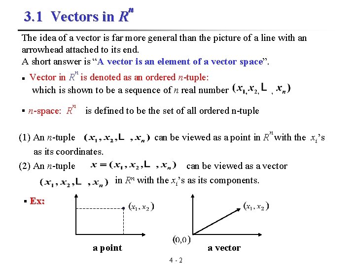
n 3. 1 Vectors in R The idea of a vector is far more general than the picture of a line with an arrowhead attached to its end. A short answer is “A vector is an element of a vector space”. n n Vector in R is denoted as an ordered n-tuple: which is shown to be a sequence of n real number § n-space: R n is defined to be the set of all ordered n-tuple n (1) An n-tuple can be viewed as a point in R with the xi’s as its coordinates. (2) An n-tuple can be viewed as a vector in Rn with the xi’s as its components. § Ex: a point a vector 4 - 2

Note: A vector space is some set of things for which the operation of addition things and the operation of multiplication by a scalar are defined. You don’t necessarily have to be able to multiply two vectors by each other or even to be able to define the length of a vector, though those are very useful operations. The common example of directed line segments (arrows) in 2 D or 3 D fits this idea, because you can add such arrows by the parallelogram law and you can multiply them by numbers, changing their length (and reversing direction for negative numbers). 4 - 3

n A complete definition of a vector space requires pinning down these properties of the operators and making the concept of vector space less vague. A vector space is a set whose elements are called “vectors” vectors and such that there are two operations defined on them: you can add vectors to each other and you can multiply them by scalars (numbers). These operations must obey certain simple rules, the axioms for a vector space. axioms 4 - 4

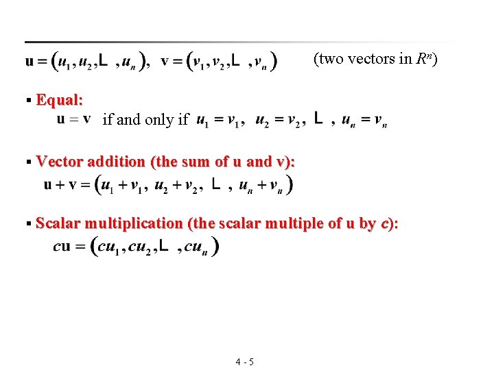
(two vectors in Rn) § Equal: if and only if § Vector addition (the sum of u and v): § Scalar multiplication (the scalar multiple of u by c): 4 - 5

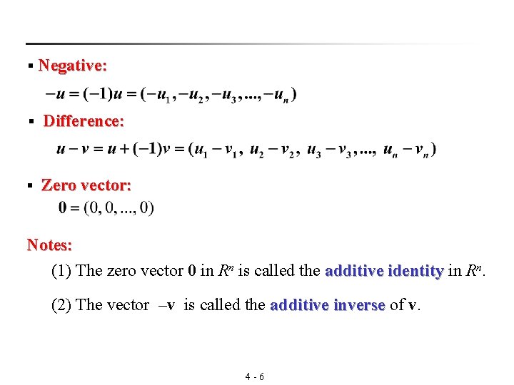
§ Negative: § Difference: § Zero vector: Notes: n. (1) The zero vector 0 in Rn is called the additive identity in R identity (2) The vector –v is called the additive inverse of v. inverse 4 - 6

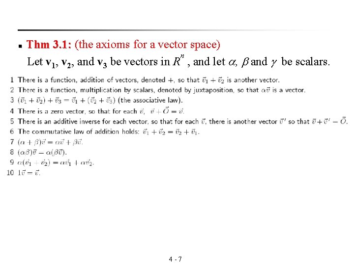
Thm 3. 1: (the axioms for a vector space) 3. 1: n Let v 1, v 2, and v 3 be vectors in R , and let , and be scalars. n 4 - 7

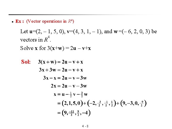
n 4) Ex : (Vector operations in R : Let u=(2, – 1, 5, 0), v=(4, 3, 1, – 1), and w=(– 6, 2, 0, 3) be 4 vectors in R. Solve x for 3(x+w) = 2 u – v+x Sol: 4 - 8

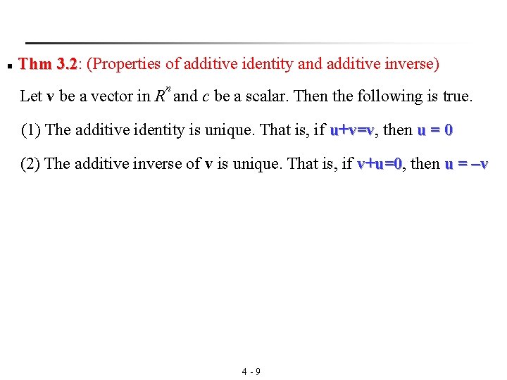
n Thm 3. 2: (Properties of additive identity and additive inverse) 3. 2 n Let v be a vector in R and c be a scalar. Then the following is true. (1) The additive identity is unique. That is, if u+v=v, then u=0 u+v=v (2) The additive inverse of v is unique. That is, if v+u=0, then u = –v v+u=0 4 - 9

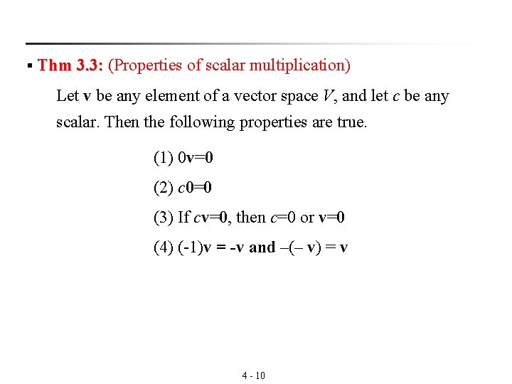
§ Thm 3. 3: (Properties of scalar multiplication) 3. 3: Let v be any element of a vector space V, and let c be any scalar. Then the following properties are true. (1) 0 v=0 (2) c 0=0 (3) If cv=0, then c=0 or v=0 (4) (-1)v = -v and –(– v) = v 4 - 10

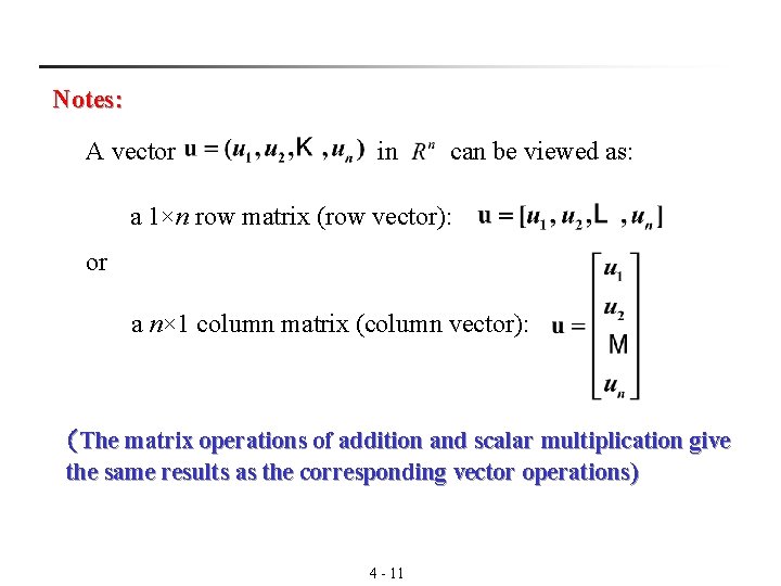
Notes: A vector in can be viewed as: a 1×n row matrix (row vector): or a n× 1 column matrix (column vector): (The matrix operations of addition and scalar multiplication give the same results as the corresponding vector operations) 4 - 11

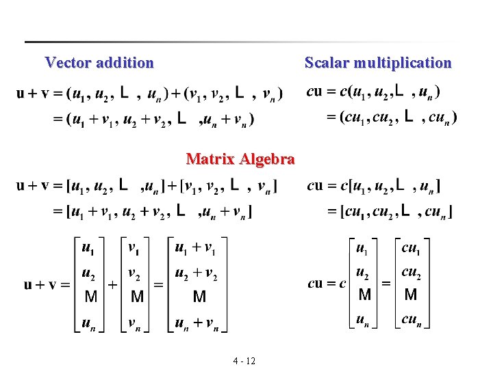
Vector addition Scalar multiplication Matrix Algebra 4 - 12

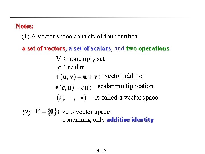
Notes: (1) A vector space consists of four entities: a set of vectors, two operations vectors a set of scalars, and scalars V:nonempty set c:scalar vector addition scalar multiplication is called a vector space (2) zero vector space containing only additive identity 4 - 13

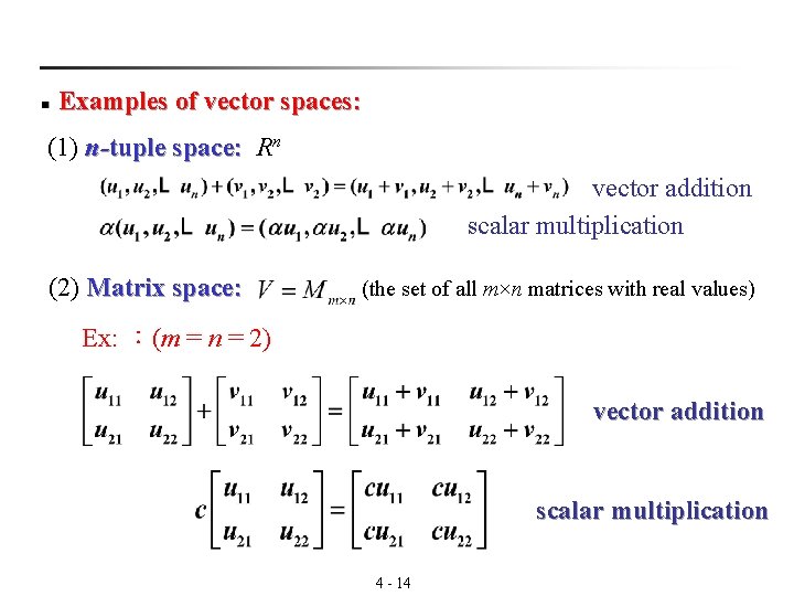
n Examples of vector spaces: (1) n-tuple space: Rn vector addition scalar multiplication (2) Matrix space: (the set of all m×n matrices with real values) Ex: :(m = n = 2) vector addition scalar multiplication 4 - 14

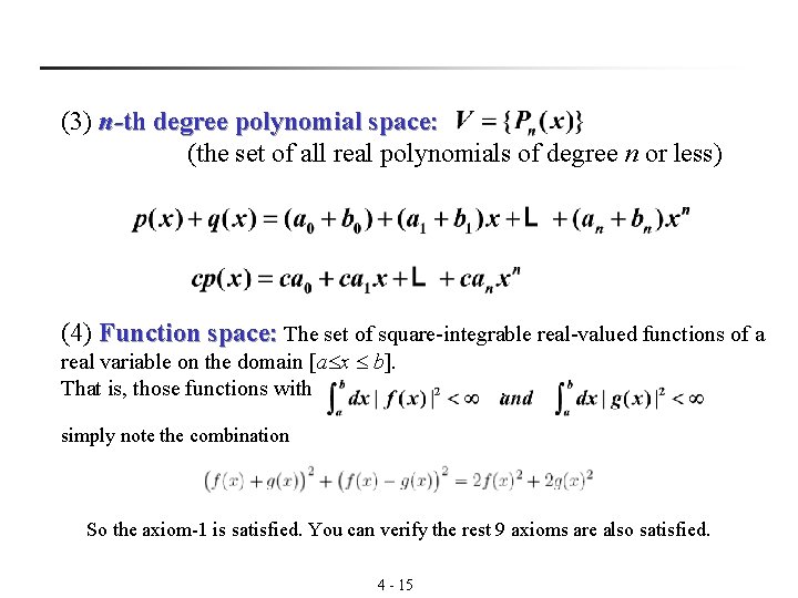
(3) n-th degree polynomial space: (the set of all real polynomials of degree n or less) (4) Function space: The set of square-integrable real-valued functions of a real variable on the domain [a x b]. That is, those functions with . simply note the combination So the axiom-1 is satisfied. You can verify the rest 9 axioms are also satisfied. 4 - 15

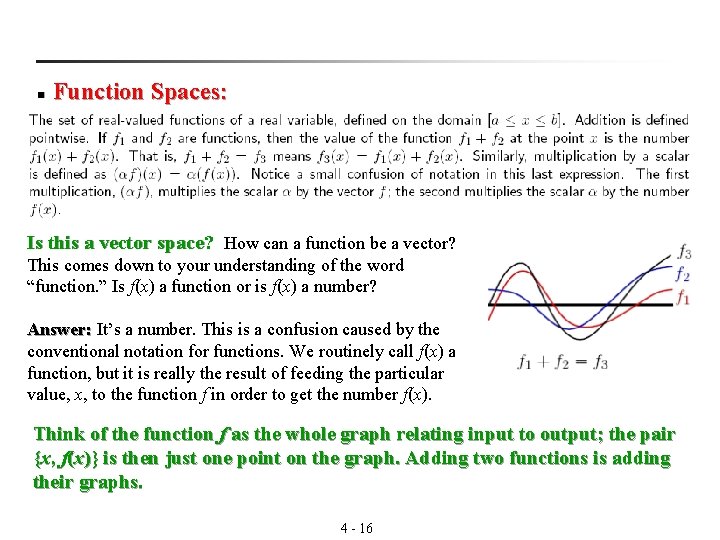
n Function Spaces: Is this a vector space? How can a function be a vector? This comes down to your understanding of the word “function. ” Is f(x) a function or is f(x) a number? Answer: It’s a number. This is a confusion caused by the Answer: conventional notation for functions. We routinely call f(x) a function, but it is really the result of feeding the particular value, x, to the function f in order to get the number f(x). Think of the function f as the whole graph relating input to output; the pair {x, f(x)} is then just one point on the graph. Adding two functions is adding their graphs. 4 - 16

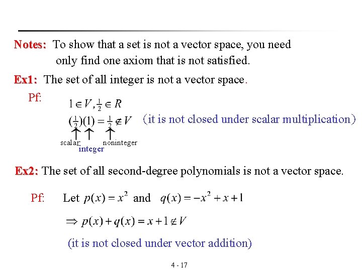
Notes: To show that a set is not a vector space, you need Notes: only find one axiom that is not satisfied. Ex 1: The set of all integer is not a vector space. Ex 1: Pf: (it is not closed under scalar multiplication) scalar noninteger Ex 2: The set of all second-degree polynomials is not a vector space. Ex 2: Pf: Let and (it is not closed under vector addition) 4 - 17

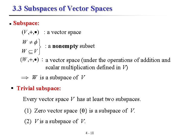
3. 3 Subspaces of Vector Spaces n Subspace: : a vector space : a nonempty subset :a vector space (under the operations of addition and scalar multiplication defined in V) W is a subspace of V § Trivial subspace: Every vector space V has at least two subspaces. (1) Zero vector space {0} is a subspace of V. (2) V is a subspace of V. 4 - 18

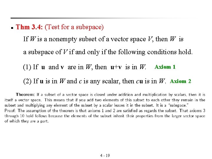
n Thm 3. 4: (Test for a subspace) 3. 4: If W is a nonempty subset of a vector space V, then W is a subspace of V if and only if the following conditions hold. (1) If u and v are in W, then u+v is in W. Axiom 1 (2) If u is in W and c is any scalar, then cu is in W. Axiom 2 4 - 19

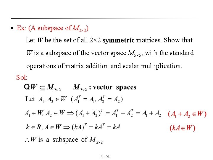
§ Ex: (A subspace of M 2× 2) Let W be the set of all 2× 2 symmetric matrices. Show that symmetric W is a subspace of the vector space M 2× 2, with the standard operations of matrix addition and scalar multiplication. Sol: 4 - 20

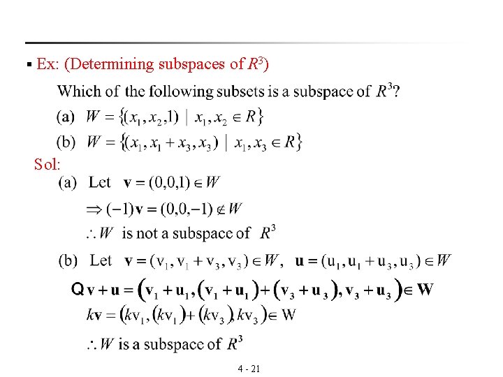
§ Ex: (Determining subspaces of R 3) Sol: 4 - 21

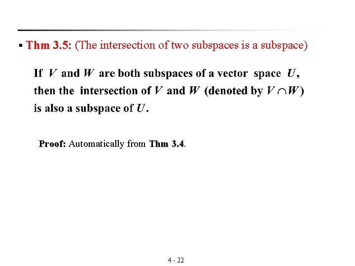
§ Thm 3. 5: (The intersection of two subspaces is a subspace) 3. 5: Proof: Automatically from Thm 3. 4. Proof: 3. 4 4 - 22

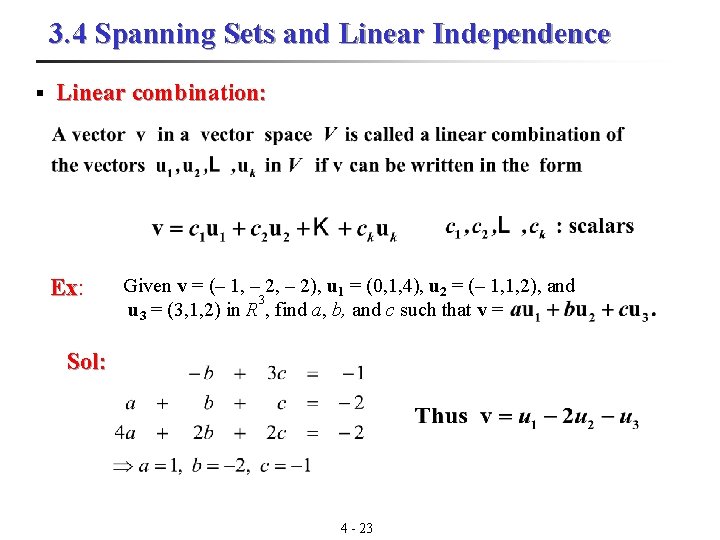
3. 4 Spanning Sets and Linear Independence § Linear combination: Ex: Ex Given v = (– 1, – 2), u 1 = (0, 1, 4), u 2 = (– 1, 1, 2), and 3 u 3 = (3, 1, 2) in R , find a, b, and c such that v = Sol: 4 - 23

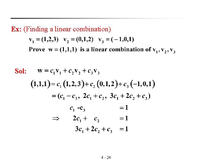
Ex: (Finding a linear combination) Ex: Sol: 4 - 24

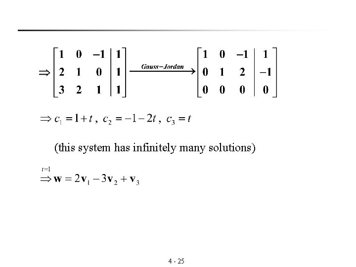
(this system has infinitely many solutions) 4 - 25

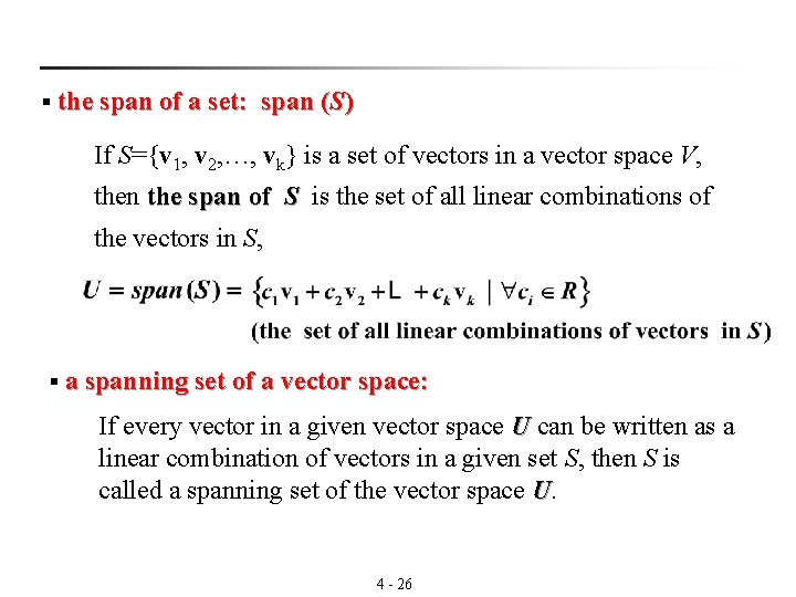
§ the span of a set: span (S) If S={v 1, v 2, …, vk} is a set of vectors in a vector space V, then the span of S is the set of all linear combinations of the vectors in S, § a spanning set of a vector space: If every vector in a given vector space U can be written as a linear combination of vectors in a given set S, then S is called a spanning set of the vector space U. 4 - 26

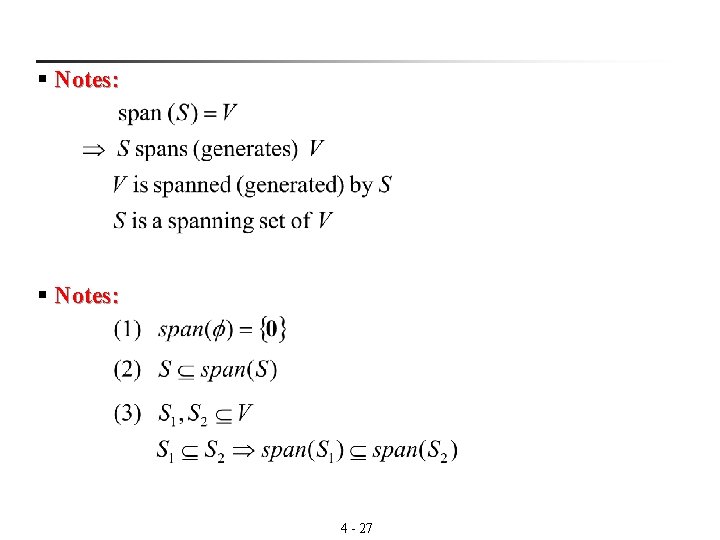
§ Notes: 4 - 27

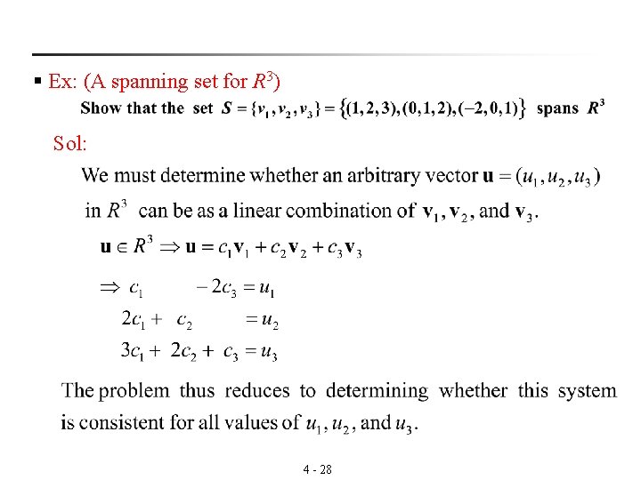
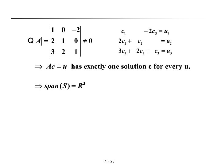
§ Ex: (A spanning set for R 3) Sol: 4 - 28

4 - 29

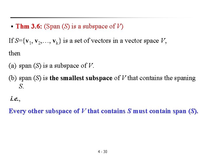
§ Thm 3. 6: (Span (S) is a subspace of V) 3. 6: If S={v 1, v 2, …, vk} is a set of vectors in a vector space V, then (a) span (S) is a subspace of V. (b) span (S) is the smallest subspace of V that contains the spaning subspace S. i. e. , Every other subspace of V that contains S must contain span (S). 4 - 30

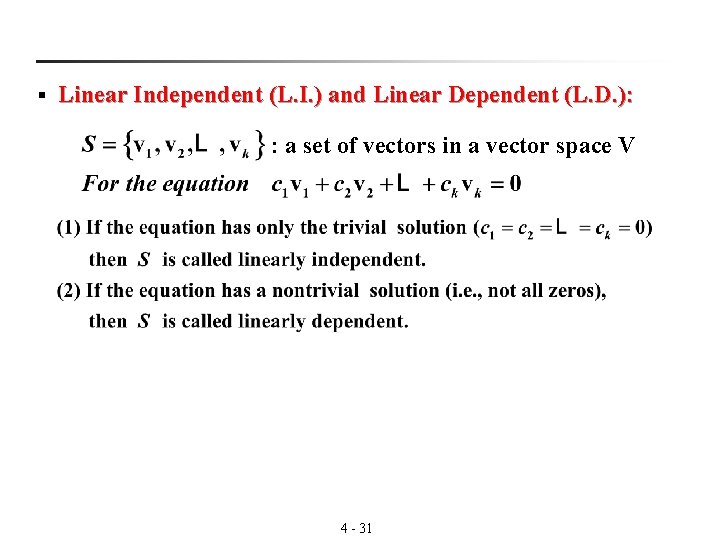
§ Linear Independent (L. I. ) and Linear Dependent (L. D. ): : a set of vectors in a vector space V 4 - 31

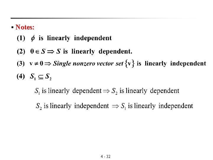
§ Notes: 4 - 32

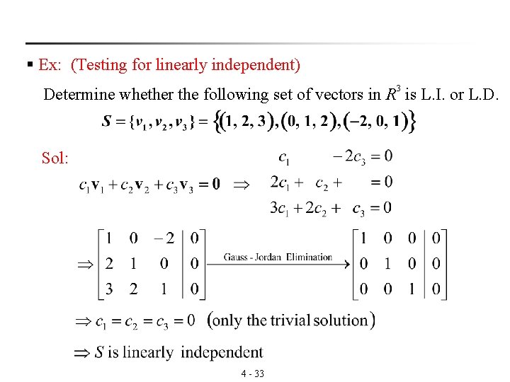
§ Ex: (Testing for linearly independent) Determine whether the following set of vectors in R 3 is L. I. or L. D. Sol: 4 - 33

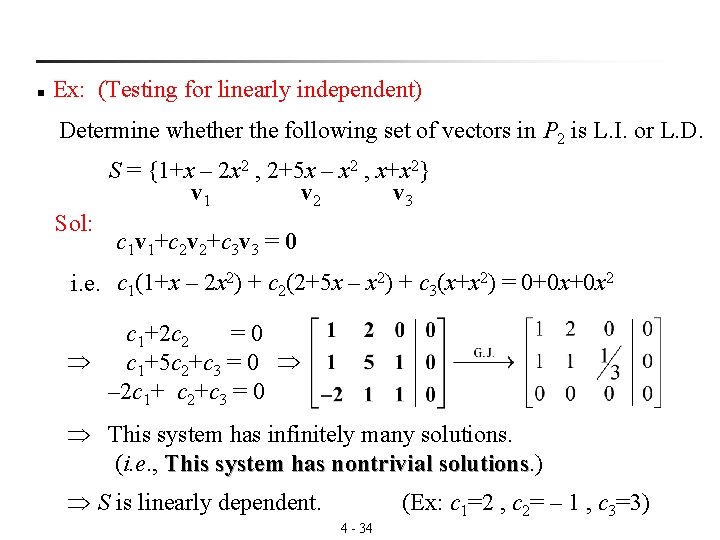
n Ex: (Testing for linearly independent) Determine whether the following set of vectors in P 2 is L. I. or L. D. S = {1+x – 2 x 2 , 2+5 x – x 2 , x+x 2} v 1 v 2 v 3 Sol: c 1 v 1+c 2 v 2+c 3 v 3 = 0 i. e. c 1(1+x – 2 x 2) + c 2(2+5 x – x 2) + c 3(x+x 2) = 0+0 x+0 x 2 c 1+2 c 2 = 0 c 1+5 c 2+c 3 = 0 – 2 c 1+ c 2+c 3 = 0 This system has infinitely many solutions. (i. e. , This system has nontrivial solutions. ) solutions S is linearly dependent. (Ex: c 1=2 , c 2= – 1 , c 3=3) 4 - 34

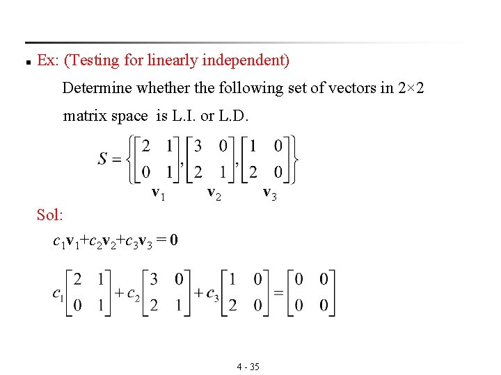
n Ex: (Testing for linearly independent) Determine whether the following set of vectors in 2× 2 matrix space is L. I. or L. D. v 1 v 2 v 3 Sol: c 1 v 1+c 2 v 2+c 3 v 3 = 0 4 - 35

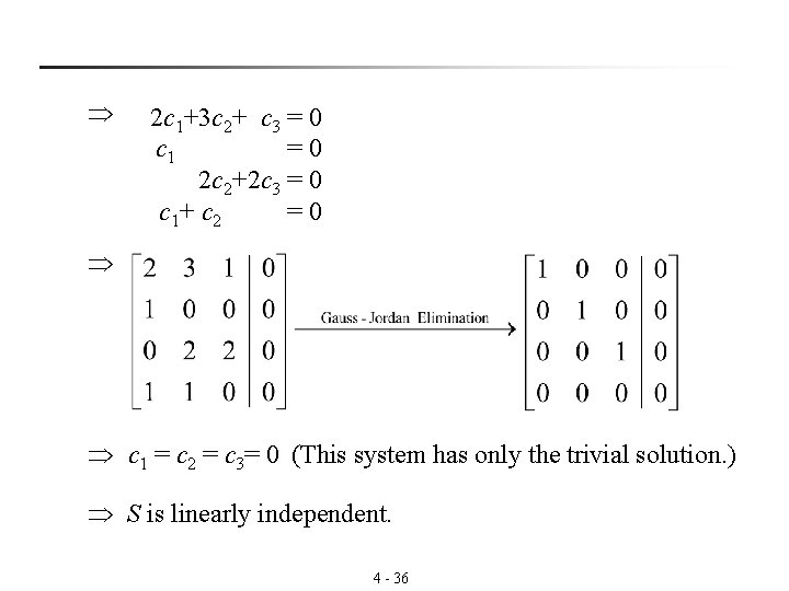
2 c 1+3 c 2+ c 3 = 0 c 1 = 0 2 c 2+2 c 3 = 0 c 1+ c 2 = 0 c 1 = c 2 = c 3= 0 (This system has only the trivial solution. ) S is linearly independent. 4 - 36

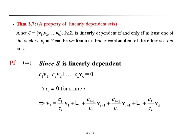
n Thm 3. 7: (A property of linearly dependent sets) 3. 7: A set S = {v 1, v 2, …, vk}, k 2, is linearly dependent if and only if at least one of the vectors vj in S can be written as a linear combination of the other vectors in S. Pf: c 1 v 1+c 2 v 2+…+ckvk = 0 ci 0 for some i 4 - 37

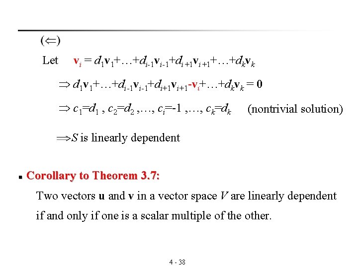
Let vi = d 1 v 1+…+di-1 vi-1+di+1 vi+1+…+dkvk d 1 v 1+…+di-1 vi-1+di+1 vi+1 -vi+…+dkvk = 0 c 1=d 1 , c 2=d 2 , …, ci=-1 , …, ck=dk (nontrivial solution) S is linearly dependent n Corollary to Theorem 3. 7: Two vectors u and v in a vector space V are linearly dependent if and only if one is a scalar multiple of the other. 4 - 38

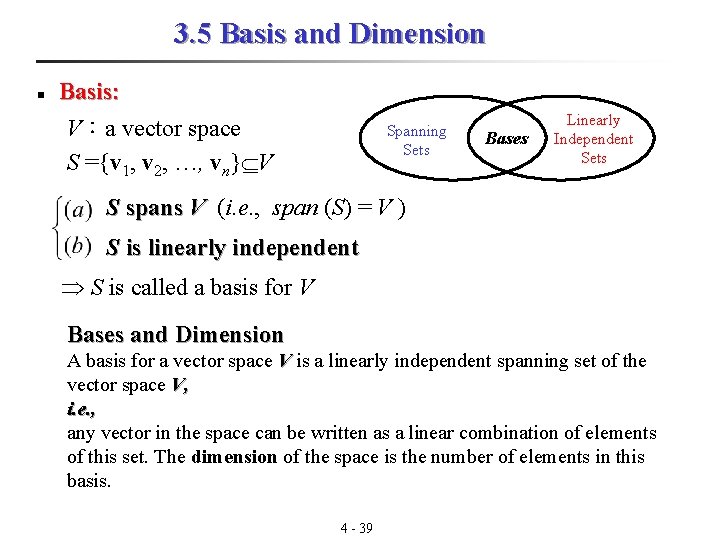
3. 5 Basis and Dimension n Basis: V:a vector space S ={v 1, v 2, …, vn} V Spanning Sets Bases Linearly Independent Sets S spans V (i. e. , span (S) = V ) S is linearly independent S is called a basis for V Bases and Dimension A basis for a vector space V is a linearly independent spanning set of the vector space V, i. e. , any vector in the space can be written as a linear combination of elements of this set. The dimension of the space is the number of elements in this basis. 4 - 39

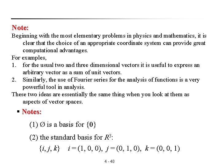
Note: Beginning with the most elementary problems in physics and mathematics, it is clear that the choice of an appropriate coordinate system can provide great computational advantages. For examples, 1. for the usual two and three dimensional vectors it is useful to express an arbitrary vector as a sum of unit vectors. 2. Similarly, the use of Fourier series for the analysis of functions is a very powerful tool in analysis. These two ideas are essentially the same thing when you look at them as aspects of vector spaces. § Notes: (1) Ø is a basis for {0} (2) the standard basis for R 3: {i, j, k} i = (1, 0, 0), j = (0, 1, 0), k = (0, 0, 1) 4 - 40

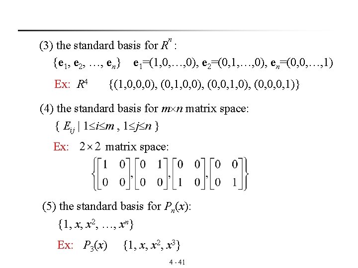
n (3) the standard basis for R : {e 1, e 2, …, en} e 1=(1, 0, …, 0), e 2=(0, 1, …, 0), en=(0, 0, …, 1) Ex: R 4 {(1, 0, 0, 0), (0, 1, 0, 0), (0, 0, 1, 0), (0, 0, 0, 1)} (4) the standard basis for m n matrix space: { Eij | 1 i m , 1 j n } Ex: matrix space: (5) the standard basis for Pn(x): {1, x, x 2, …, xn} Ex: P 3(x) {1, x, x 2, x 3} 4 - 41

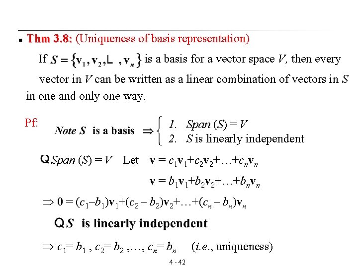
n Thm 3. 8: (Uniqueness of basis representation) 3. 8: If is a basis for a vector space V, then every vector in V can be written as a linear combination of vectors in S in one and only one way. Pf: 1. Span (S) = V 2. S is linearly independent Span (S) = V Let v = c 1 v 1+c 2 v 2+…+cnvn v = b 1 v 1+b 2 v 2+…+bnvn 0 = (c 1–b 1)v 1+(c 2 – b 2)v 2+…+(cn – bn)vn c 1= b 1 , c 2= b 2 , …, cn= bn 4 - 42 (i. e. , uniqueness)

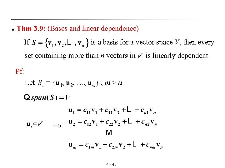
n Thm 3. 9: (Bases and linear dependence) 3. 9: If is a basis for a vector space V, then every set containing more than n vectors in V is linearly dependent. Pf: Let S 1 = {u 1, u 2, …, um} , m > n ui V 4 - 43

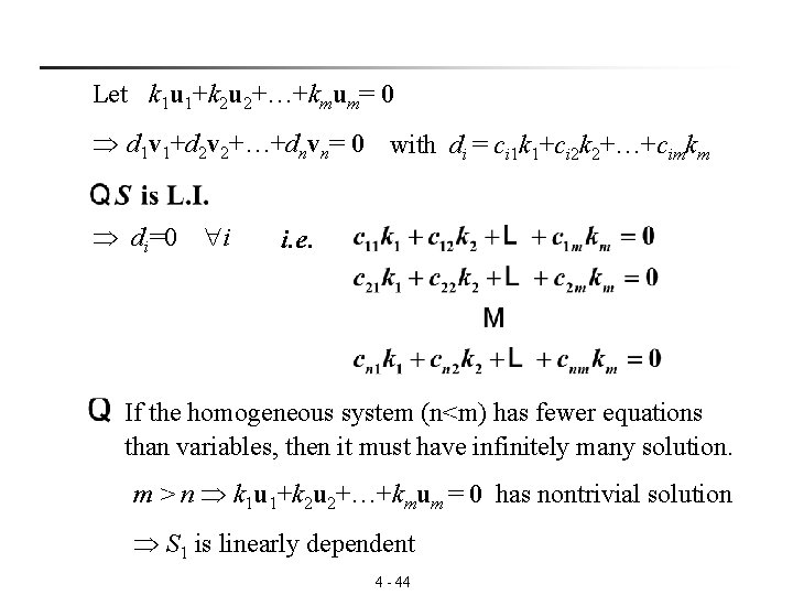
Let k 1 u 1+k 2 u 2+…+kmum= 0 d 1 v 1+d 2 v 2+…+dnvn= 0 with di = ci 1 k 1+ci 2 k 2+…+cimkm di=0 i i. e. If the homogeneous system (n<m) has fewer equations than variables, then it must have infinitely many solution. m > n k 1 u 1+k 2 u 2+…+kmum = 0 has nontrivial solution S 1 is linearly dependent 4 - 44

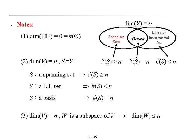
§ dim(V) = n Notes: (1) dim({0}) = 0 = #(Ø) Spanning Sets (2) dim(V) = n , S V #(S) > n Bases Linearly Independent Sets #(S) = n #(S) < n S:a spanning set #(S) n S:a L. I. set #(S) n S:a basis #(S) = n (3) dim(V) = n , W is a subspace of V dim(W) n 4 - 45

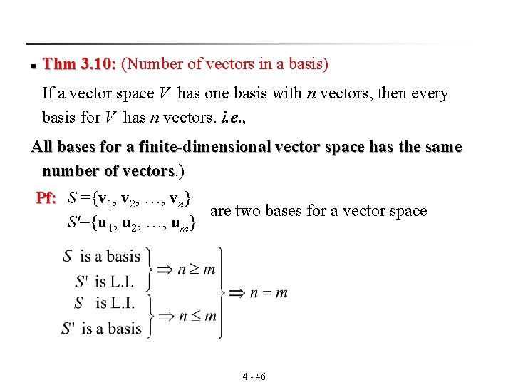
n Thm 3. 10: (Number of vectors in a basis) 3. 10: If a vector space V has one basis with n vectors, then every basis for V has n vectors. i. e. , All bases for a finite-dimensional vector space has the same number of vectors. ) vectors Pf: S ={v 1, v 2, …, vn} are two bases for a vector space S'={u 1, u 2, …, um} 4 - 46

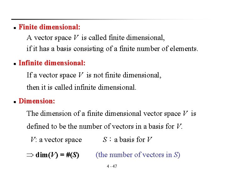
Finite dimensional: A vector space V is called finite dimensional, if it has a basis consisting of a finite number of elements. n n Infinite dimensional: If a vector space V is not finite dimensional, then it is called infinite dimensional. n Dimension: The dimension of a finite dimensional vector space V is defined to be the number of vectors in a basis for V. V: a vector space dim(V) = #(S) S:a basis for V (the number of vectors in S) 4 - 47

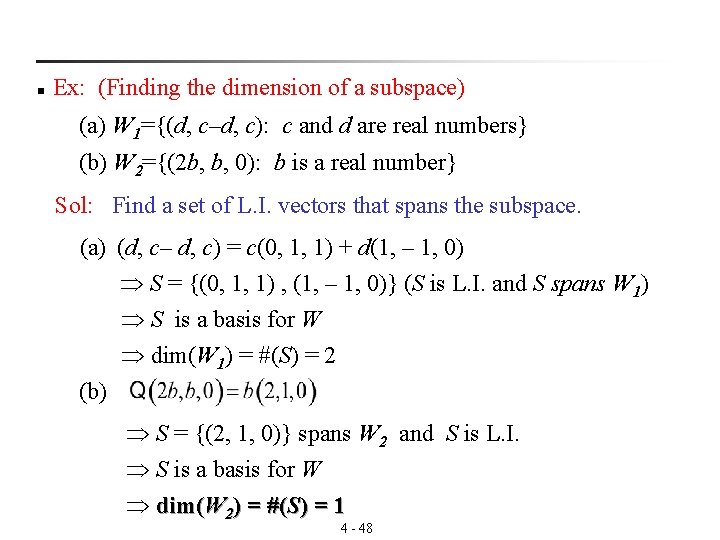
n Ex: (Finding the dimension of a subspace) (a) W 1={(d, c–d, c): c and d are real numbers} (b) W 2={(2 b, b, 0): b is a real number} Sol: Find a set of L. I. vectors that spans the subspace. (a) (d, c– d, c) = c(0, 1, 1) + d(1, – 1, 0) S = {(0, 1, 1) , (1, – 1, 0)} (S is L. I. and S spans W 1) S is a basis for W dim(W 1) = #(S) = 2 (b) S = {(2, 1, 0)} spans W 2 and S is L. I. S is a basis for W dim(W 2) = #(S) = 1 4 - 48

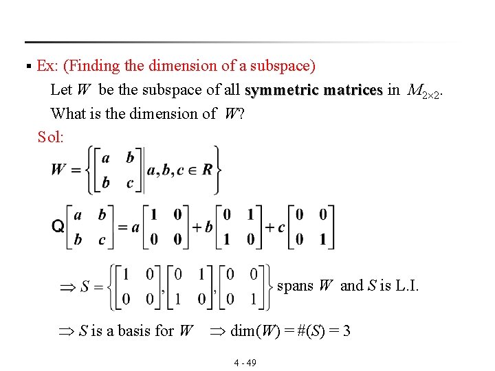
Ex: (Finding the dimension of a subspace) Let W be the subspace of all symmetric matrices in M matrices 2 2. What is the dimension of W? Sol: § spans W and S is L. I. S is a basis for W dim(W) = #(S) = 3 4 - 49

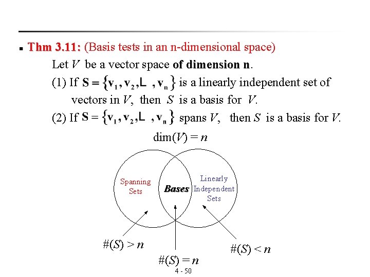
Thm 3. 11: (Basis tests in an n-dimensional space) 3. 11: Let V be a vector space of dimension n. n (1) If is a linearly independent set of vectors in V, then S is a basis for V. (2) If spans V, then S is a basis for V. n dim(V) = n Spanning Sets Bases Linearly Independent Sets #(S) > n #(S) = n 4 - 50 #(S) < n

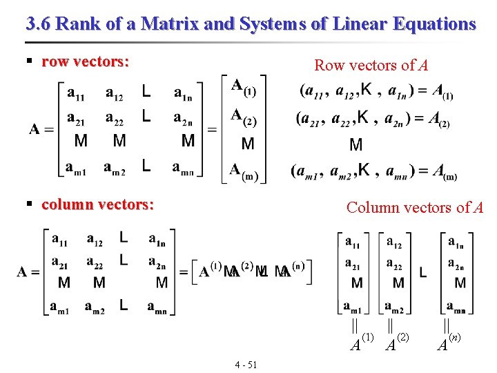
3. 6 Rank of a Matrix and Systems of Linear Equations § row vectors: Row vectors of A § column vectors: Column vectors of A || || (1) (2) (n) A A A 4 - 51

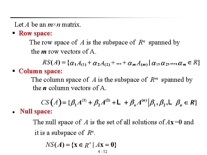
Let A be an m×n matrix. § Row space: The row space of A is the subspace of Rn spanned by the m row vectors of A. § Column space: The column space of A is the subspace of Rm spanned by the n column vectors of A. Null space: n The null space of A is the set of all solutions of Ax=0 and it is a subspace of Rn. 4 - 52

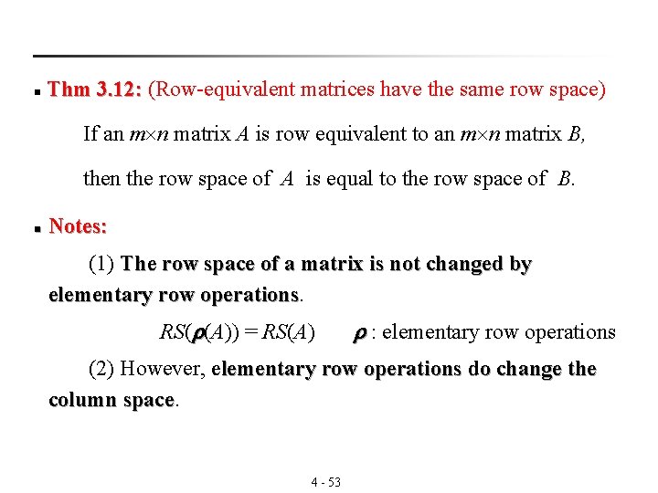
Thm 3. 12: (Row-equivalent matrices have the same row space) 3. 12: n If an m n matrix A is row equivalent to an m n matrix B, then the row space of A is equal to the row space of B. n Notes: (1) The row space of a matrix is not changed by elementary row operations RS( (A)) = RS(A) : elementary row operations (2) However, elementary row operations do change the column space 4 - 53

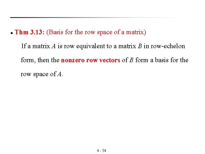
n Thm 3. 13: (Basis for the row space of a matrix) 3. 13: If a matrix A is row equivalent to a matrix B in row-echelon form, then the nonzero row vectors of B form a basis for the vectors row space of A. 4 - 54

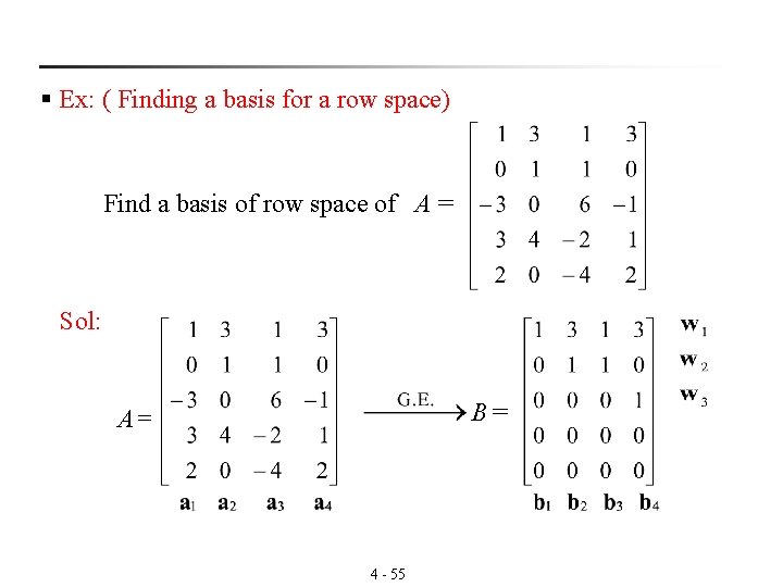
§ Ex: ( Finding a basis for a row space) Find a basis of row space of A = Sol: B = A= 4 - 55

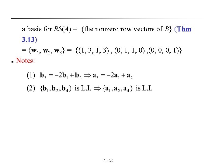
n a basis for RS(A) = {the nonzero row vectors of B} (Thm 3. 13) 3. 13 = {w 1, w 2, w 3} = {(1, 3, 1, 3) , (0, 1, 1, 0) , (0, 0, 0, 1)} Notes: 4 - 56

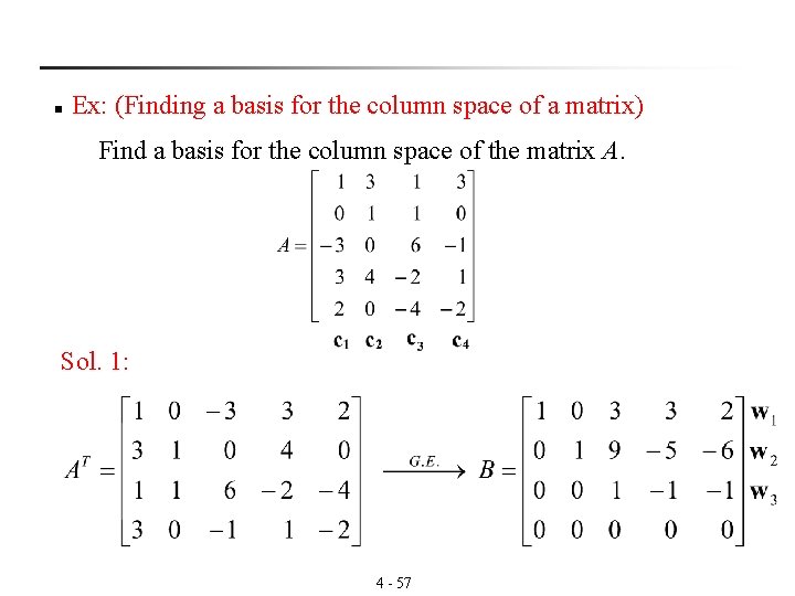
n Ex: (Finding a basis for the column space of a matrix) Find a basis for the column space of the matrix A. Sol. 1: 4 - 57

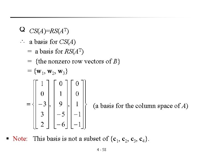
CS(A)=RS(AT) a basis for CS(A) = a basis for RS(AT) = {the nonzero row vectors of B} = {w 1, w 2, w 3} (a basis for the column space of A) § Note: This basis is not a subset of {c 1, c 2, c 3, c 4}. 4 - 58

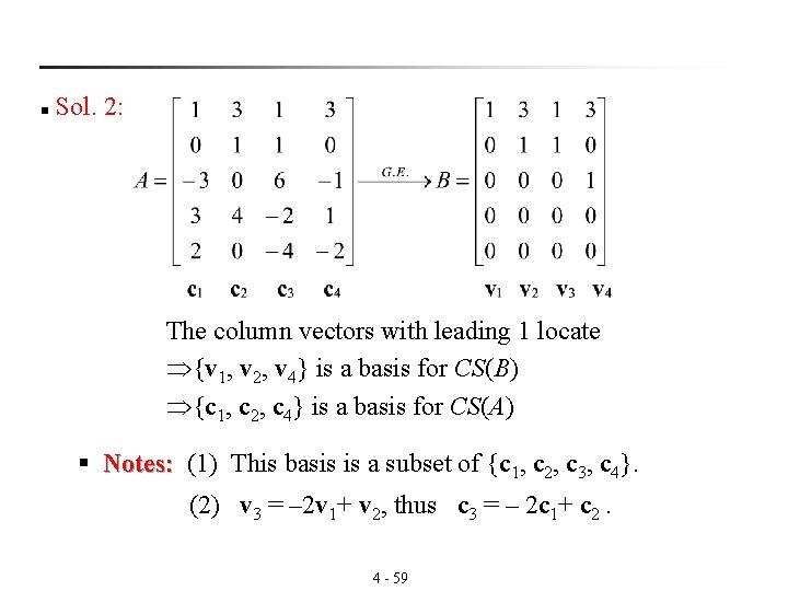
Sol. 2: n The column vectors with leading 1 locate {v 1, v 2, v 4} is a basis for CS(B) {c 1, c 2, c 4} is a basis for CS(A) § Notes: (1) This basis is a subset of {c Notes: 1, c 2, c 3, c 4}. (2) v 3 = – 2 v 1+ v 2, thus c 3 = – 2 c 1+ c 2. 4 - 59

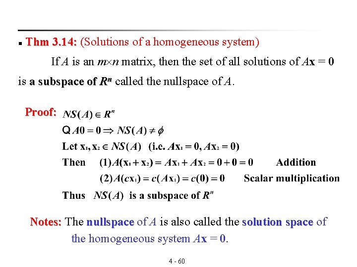
Thm 3. 14: (Solutions of a homogeneous system) 3. 14: n If A is an m n matrix, then the set of all solutions of Ax = 0 is a subspace of Rn called the nullspace of A. Proof: Notes: The nullspace of A is also called the solution space of Notes: nullspace the homogeneous system Ax = 0. 4 - 60

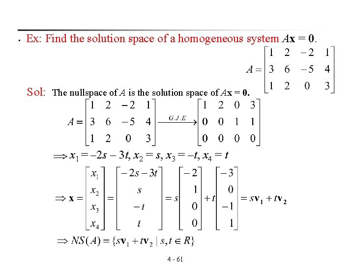
§ Ex: Find the solution space of a homogeneous system Ax = 0. Sol: The nullspace of A is the solution space of Ax = 0. x 1 = – 2 s – 3 t, x 2 = s, x 3 = –t, x 4 = t 4 - 61

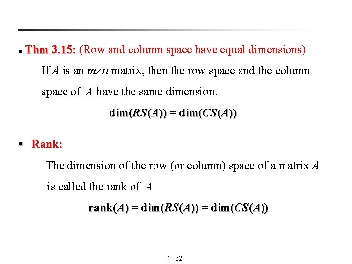
Thm 3. 15: (Row and column space have equal dimensions) 3. 15: n If A is an m n matrix, then the row space and the column space of A have the same dimension. dim(RS(A)) = dim(CS(A)) § Rank: The dimension of the row (or column) space of a matrix A is called the rank of A. rank(A) = dim(RS(A)) = dim(CS(A)) 4 - 62

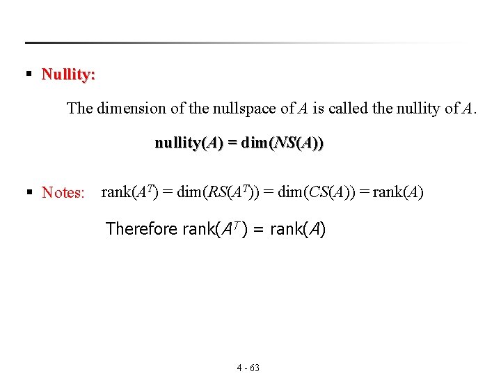
§ Nullity: The dimension of the nullspace of A is called the nullity of A. nullity(A) = dim(NS(A)) § Notes: rank(AT) = dim(RS(AT)) = dim(CS(A)) = rank(A) Therefore rank(AT ) = rank(A) 4 - 63

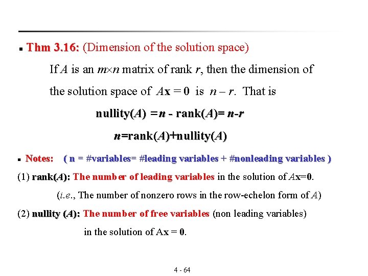
Thm 3. 16: (Dimension of the solution space) 3. 16: n If A is an m n matrix of rank r, then the dimension of the solution space of Ax = 0 is n – r. That is nullity(A) =n - rank(A)= n-r n=rank(A)+nullity(A) n Notes: ( n = #variables= #leading variables + #nonleading variables ) (1) rank(A): The number of leading variables in the solution of Ax=0. ): (i. e. , The number of nonzero rows in the row-echelon form of A) (2) nullity (A): The number of free variables (non leading variables) ): in the solution of Ax = 0. 4 - 64

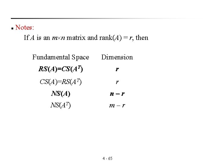
Notes: If A is an m n matrix and rank(A) = r, then n Fundamental Space Dimension RS(A)=CS(AT) r CS(A)=RS(AT) r NS(A) n–r NS(AT) m–r 4 - 65

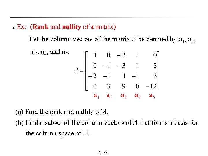
n Ex: (Rank and nullity of a matrix) Rank nullity Let the column vectors of the matrix A be denoted by a 1, a 2, a 3, a 4, and a 5. a 1 a 2 a 3 a 4 a 5 (a) Find the rank and nullity of A. (b) Find a subset of the column vectors of A that forms a basis for the column space of A. 4 - 66

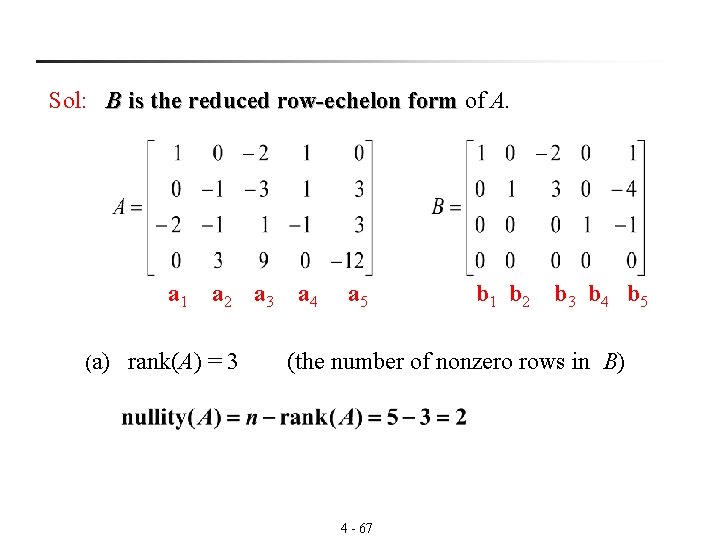
Sol: B is the reduced row-echelon form of A. form a 1 a 2 a 3 a 4 a 5 b 1 b 2 b 3 b 4 b 5 (a) rank(A) = 3 (the number of nonzero rows in B) 4 - 67

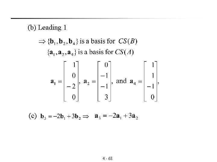
(b) Leading 1 (c) 4 - 68

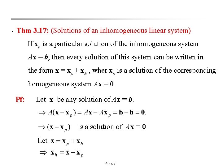
§ Thm 3. 17: (Solutions of an inhomogeneous linear system) 3. 17: If xp is a particular solution of the inhomogeneous system Ax = b, then every solution of this system can be written in the form x = xp + xh , wher xh is a solution of the corresponding homogeneous system Ax = 0. Pf: Let x be any solution of Ax = b. is a solution of Ax = 0 4 - 69

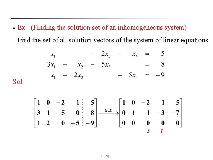
n Ex: (Finding the solution set of an inhomogeneous system) Find the set of all solution vectors of the system of linear equations. Sol: s 4 - 70 t

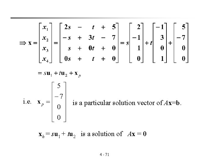
i. e. is a particular solution vector of Ax=b. xh = su 1 + tu 2 is a solution of Ax = 0 4 - 71

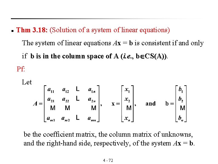
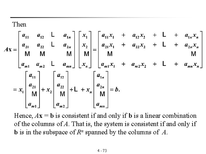
n Thm 3. 18: (Solution of a system of linear equations) 3. 18: The system of linear equations Ax = b is consistent if and only if b is in the column space of A (i. e. , b CS(A)). Pf: Let be the coefficient matrix, the column matrix of unknowns, and the right-hand side, respectively, of the system Ax = b. 4 - 72

Then Hence, Ax = b is consistent if and only if b is a linear combination of the columns of A. That is, the system is consistent if and only if b is in the subspace of Rn spanned by the columns of A. 4 - 73
![Notes If rankAbrankA Thm 3 18 3 18 Then the system Axb is § Notes: If rank([A|b])=rank(A) (Thm 3. 18) 3. 18 Then the system Ax=b is](https://slidetodoc.com/presentation_image_h/e2bff8f0f6d568359f3121bfb16656c4/image-74.jpg)
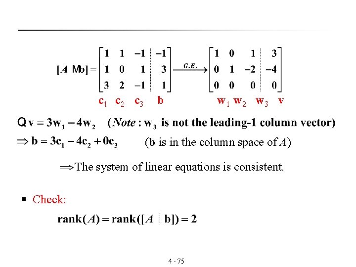
§ Notes: If rank([A|b])=rank(A) (Thm 3. 18) 3. 18 Then the system Ax=b is consistent. n Ex: (Consistency of a system of linear equations) Sol: 4 - 74

c 1 c 2 c 3 b w 1 w 2 w 3 v (b is in the column space of A) The system of linear equations is consistent. § Check: 4 - 75

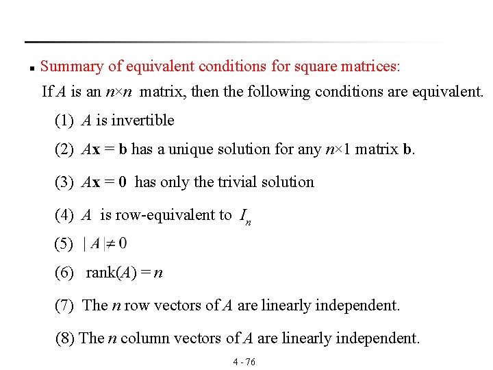
n Summary of equivalent conditions for square matrices: If A is an n×n matrix, then the following conditions are equivalent. (1) A is invertible (2) Ax = b has a unique solution for any n× 1 matrix b. (3) Ax = 0 has only the trivial solution (4) A is row-equivalent to In (5) (6) rank(A) = n (7) The n row vectors of A are linearly independent. (8) The n column vectors of A are linearly independent. 4 - 76

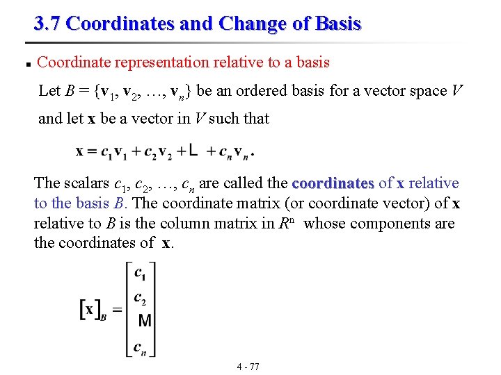
3. 7 Coordinates and Change of Basis n Coordinate representation relative to a basis Let B = {v 1, v 2, …, vn} be an ordered basis for a vector space V and let x be a vector in V such that The scalars c 1, c 2, …, cn are called the coordinates of x relative coordinates to the basis B. The coordinate matrix (or coordinate vector) of x relative to B is the column matrix in Rn whose components are the coordinates of x. 4 - 77

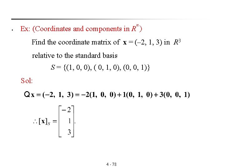
n § Ex: (Coordinates and components in R ) Find the coordinate matrix of x = (– 2, 1, 3) in R 3 relative to the standard basis S = {(1, 0, 0), ( 0, 1, 0), (0, 0, 1)} Sol: 4 - 78

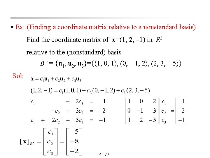
§ Ex: (Finding a coordinate matrix relative to a nonstandard basis) Find the coordinate matrix of x=(1, 2, – 1) in R 3 relative to the (nonstandard) basis B ' = {u 1, u 2, u 3}={(1, 0, 1), (0, – 1, 2), (2, 3, – 5)} Sol: 4 - 79

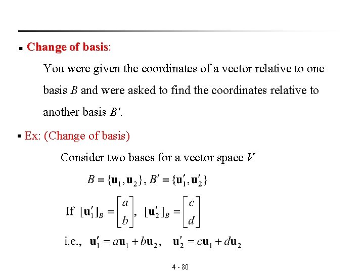
n Change of basis: basis You were given the coordinates of a vector relative to one basis B and were asked to find the coordinates relative to another basis B'. § Ex: (Change of basis) Consider two bases for a vector space V 4 - 80

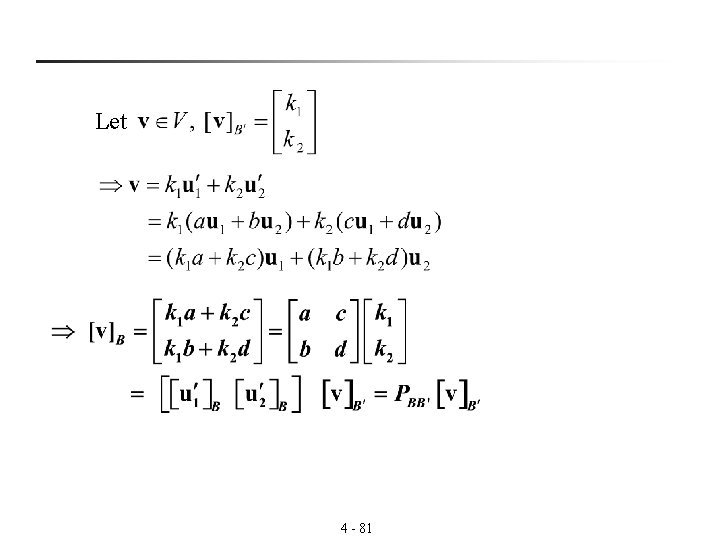
Let 4 - 81
![n Transition matrix from B to B If vB is the coordinate matrix of n Transition matrix from B' to B: If [v]B is the coordinate matrix of](https://slidetodoc.com/presentation_image_h/e2bff8f0f6d568359f3121bfb16656c4/image-82.jpg)
n Transition matrix from B' to B: If [v]B is the coordinate matrix of v relative to B [v]B’ is the coordinate matrix of v relative to B' where is called the transition matrix from B' to B matrix 4 - 82

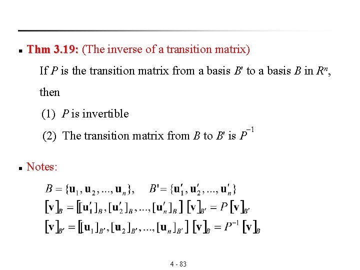
n Thm 3. 19: (The inverse of a transition matrix) 3. 19: If P is the transition matrix from a basis B' to a basis B in Rn, then (1) P is invertible (2) The transition matrix from B to B' is P n Notes: 4 - 83 – 1

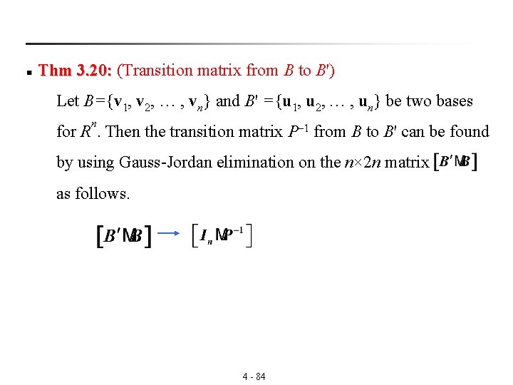
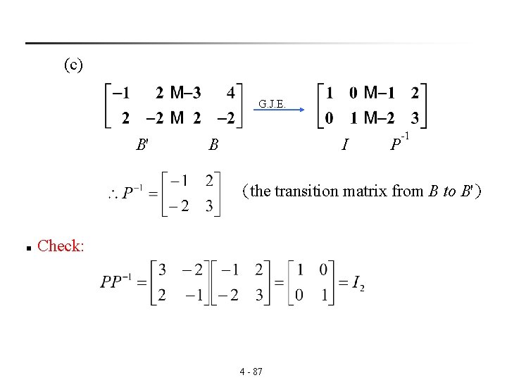
n Thm 3. 20: (Transition matrix from B to B') 3. 20: Let B={v 1, v 2, … , vn} and B' ={u 1, u 2, … , un} be two bases n for R. Then the transition matrix P– 1 from B to B' can be found by using Gauss-Jordan elimination on the n× 2 n matrix as follows. 4 - 84

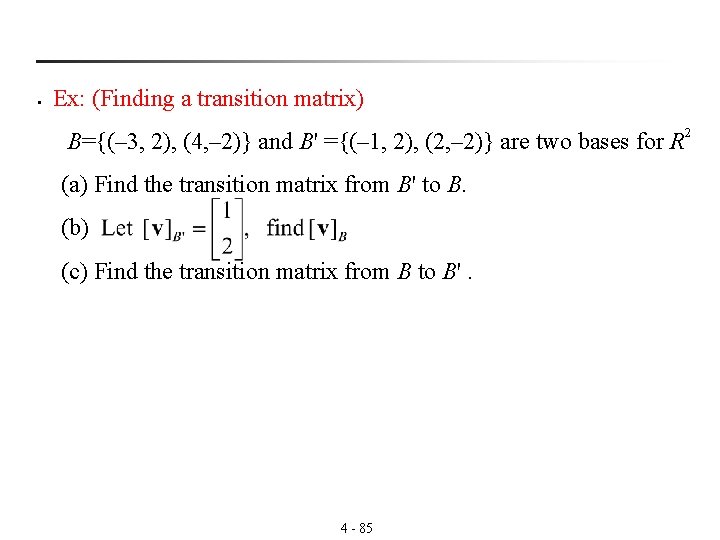
§ Ex: (Finding a transition matrix) B={(– 3, 2), (4, – 2)} and B' ={(– 1, 2), (2, – 2)} are two bases for R 2 (a) Find the transition matrix from B' to B. (b) (c) Find the transition matrix from B to B'. 4 - 85

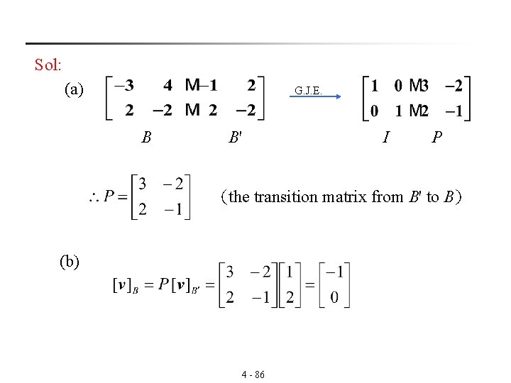
Sol: (a) G. J. E. B B' I P (the transition matrix from B' to B) (b) 4 - 86

(c) G. J. E. B' B I P -1 (the transition matrix from B to B') n Check: 4 - 87

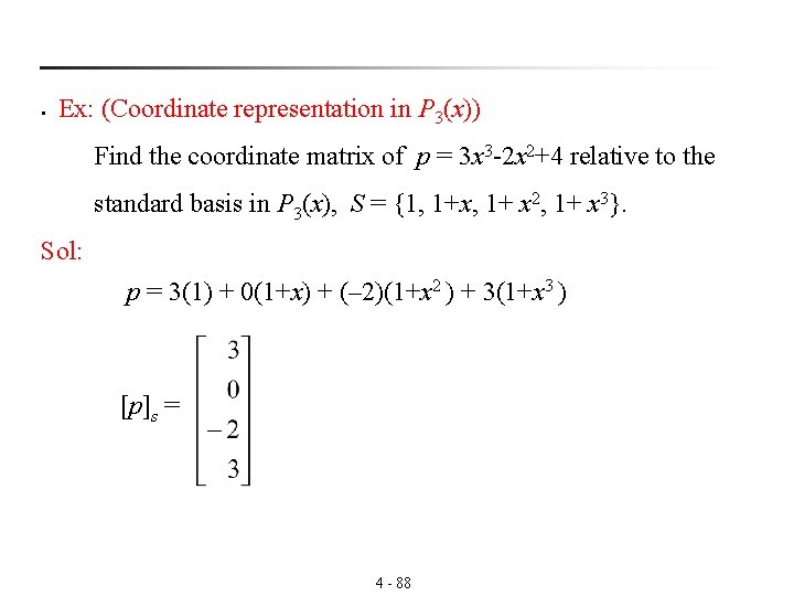
§ Ex: (Coordinate representation in P 3(x)) Find the coordinate matrix of p = 3 x 3 -2 x 2+4 relative to the standard basis in P 3(x), S = {1, 1+x, 1+ x 2, 1+ x 3}. Sol: p = 3(1) + 0(1+x) + (– 2)(1+x 2 ) + 3(1+x 3 ) [p]s = 4 - 88

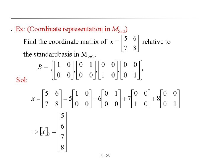
§ Ex: (Coordinate representation in M 2 x 2) Find the coordinate matrix of x = relative to the standardbasis in M 2 x 2. B = Sol: 4 - 89