Support Vector Machines Chapter 18 9 1 Support

Support Vector Machines Chapter 18. 9 1

Support Vector Machines Note to other teachers and users of these slides. Andrew would be delighted if you found this source material useful in giving your own lectures. Feel free to use these slides verbatim, or to modify them to fit your own needs. Power. Point originals are available. If you make use of a significant portion of these slides in your own lecture, please include this message, or the following link to the source repository of Andrew’s tutorials: http: //www. cs. cmu. edu/~awm/tutorials. Comments and corrections gratefully received. Andrew W. Moore Professor School of Computer Science Carnegie Mellon University www. cs. cmu. edu/~awm awm@cs. cmu. edu 412 -268 -7599 Copyright © 2001, 2003, Andrew W. Moore Nov 23 rd, 2001

Overviews • Proposed by Vapnik and his colleagues - Started in 1963, taking shape in late 70’s as part of his statistical learning theory (with Chervonenkis) - Current form established in early 90’s (with Cortes) • Becomes popular in last decade - Classification, regression (function approx. ), optimization - Compared favorably to MLP • Basic ideas - Overcoming linear seperability problem by transforming the problem into higher dimensional space using kernel functions - (become equiv. to 2 -layer perceptron when kernel is sigmoid function) - Maximize margin of decision boundary Copyright © 2001, 2003, Andrew W. Moore Support Vector Machines: Slide 3

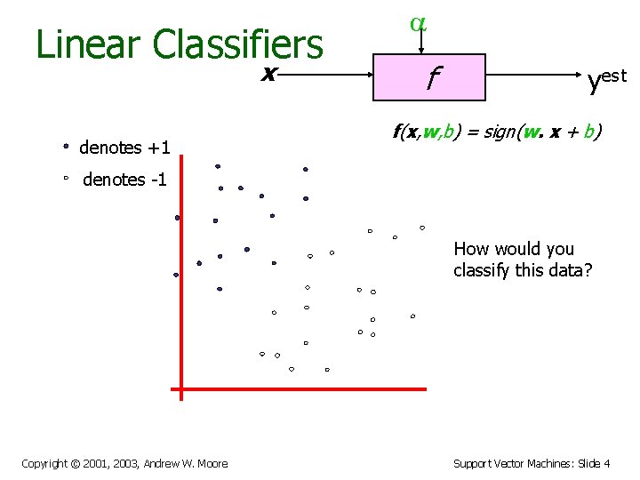
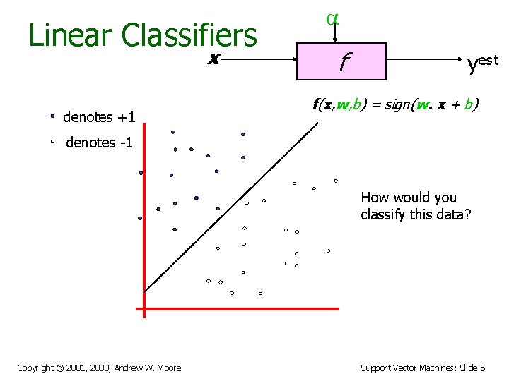
Linear Classifiers x denotes +1 a f yest f(x, w, b) = sign(w. x + b) denotes -1 How would you classify this data? Copyright © 2001, 2003, Andrew W. Moore Support Vector Machines: Slide 4

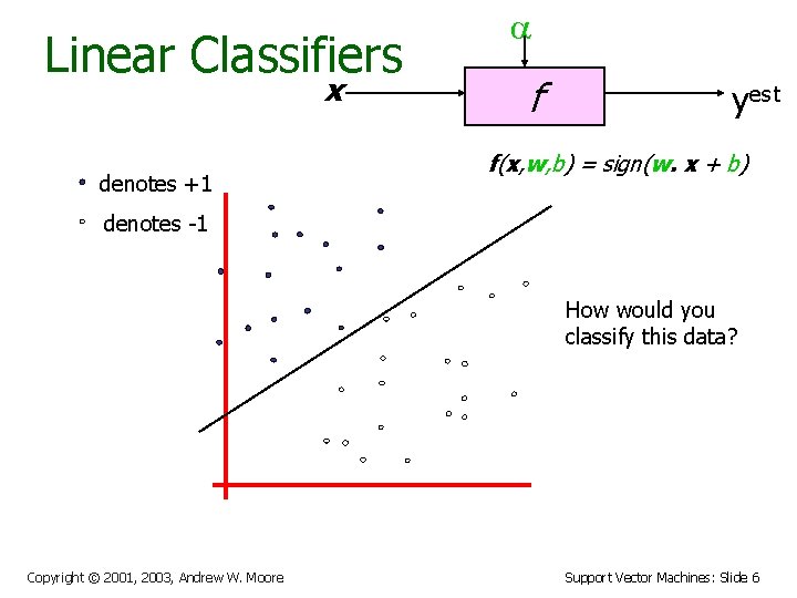
Linear Classifiers x denotes +1 a f yest f(x, w, b) = sign(w. x + b) denotes -1 How would you classify this data? Copyright © 2001, 2003, Andrew W. Moore Support Vector Machines: Slide 5

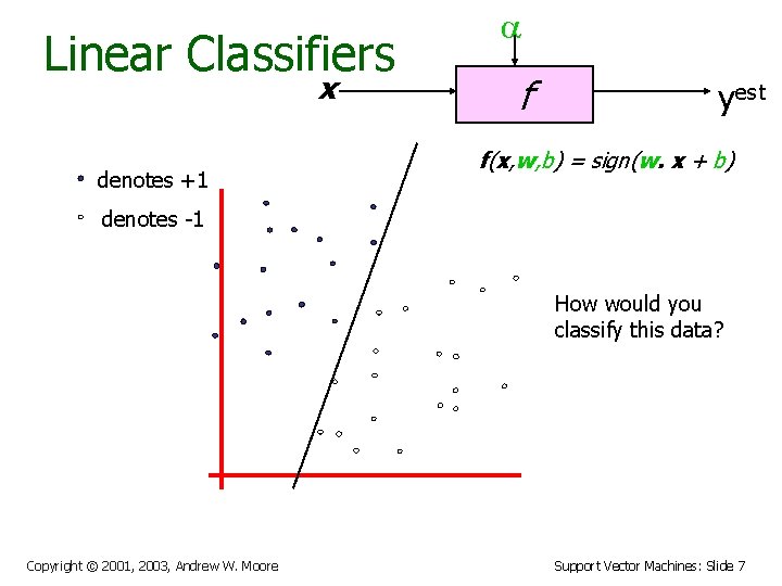
Linear Classifiers x denotes +1 a f yest f(x, w, b) = sign(w. x + b) denotes -1 How would you classify this data? Copyright © 2001, 2003, Andrew W. Moore Support Vector Machines: Slide 6

Linear Classifiers x denotes +1 a f yest f(x, w, b) = sign(w. x + b) denotes -1 How would you classify this data? Copyright © 2001, 2003, Andrew W. Moore Support Vector Machines: Slide 7

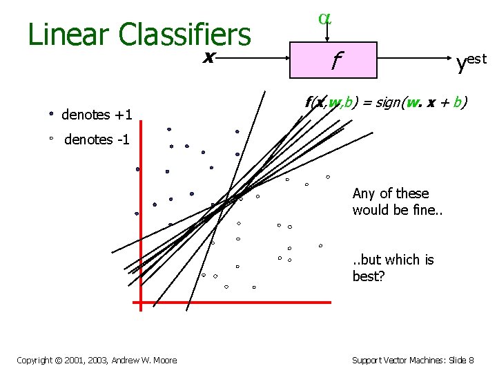
Linear Classifiers x denotes +1 a f yest f(x, w, b) = sign(w. x + b) denotes -1 Any of these would be fine. . but which is best? Copyright © 2001, 2003, Andrew W. Moore Support Vector Machines: Slide 8

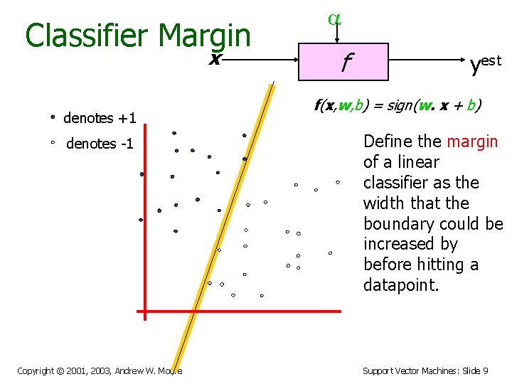
Classifier Margin x denotes +1 denotes -1 Copyright © 2001, 2003, Andrew W. Moore a f yest f(x, w, b) = sign(w. x + b) Define the margin of a linear classifier as the width that the boundary could be increased by before hitting a datapoint. Support Vector Machines: Slide 9

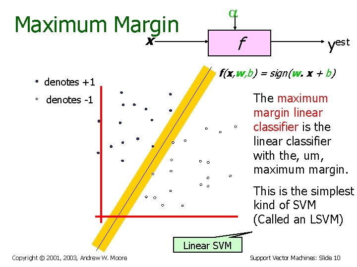
Maximum Margin a x denotes +1 f yest f(x, w, b) = sign(w. x + b) The maximum margin linear classifier is the linear classifier with the, um, maximum margin. denotes -1 This is the simplest kind of SVM (Called an LSVM) Linear SVM Copyright © 2001, 2003, Andrew W. Moore Support Vector Machines: Slide 10

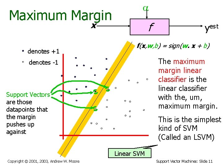
Maximum Margin a x denotes +1 f yest f(x, w, b) = sign(w. x + b) The maximum margin linear classifier is the linear classifier with the, um, maximum margin. denotes -1 Support Vectors are those datapoints that the margin pushes up against This is the simplest kind of SVM (Called an LSVM) Linear SVM Copyright © 2001, 2003, Andrew W. Moore Support Vector Machines: Slide 11

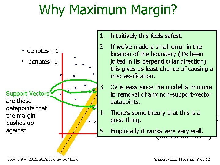
Why Maximum Margin? 1. Intuitively this feels safest. denotes +1 denotes -1 Support Vectors are those datapoints that the margin pushes up against Copyright © 2001, 2003, Andrew W. Moore f(x, w, b) = sign(w. - b) 2. If we’ve made a small error inxthe location of the boundary (it’s been The maximum jolted in its perpendicular direction) this gives us leastmargin chance linear of causing a misclassification. classifier is the 3. CV is easy since the model is immune linear classifier to removal of anywith non-support-vector the, um, datapoints. maximum margin. 4. There’s some theory that this is a This is the simplest good thing. kind of SVM (Called an LSVM) 5. Empirically it works very well. Support Vector Machines: Slide 12

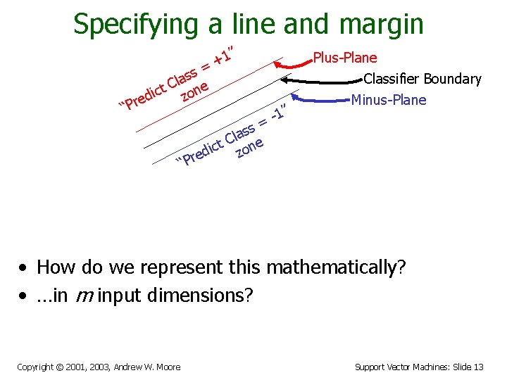
Specifying a line and margin ” 1 + = ss a l t C one c i z ed r P “ Plus-Plane Classifier Boundary 1” = Minus-Plane ss a l t C one c i z red “P • How do we represent this mathematically? • …in m input dimensions? Copyright © 2001, 2003, Andrew W. Moore Support Vector Machines: Slide 13

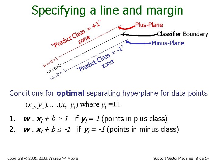
Specifying a line and margin ” 1 + = ss a l t C one c i z ed r P “ =1 b + 0 wx b= + wx b=-1 + wx Plus-Plane Classifier Boundary 1” = Minus-Plane ss a l t C one c i z red “P Conditions for optimal separating hyperplane for data points (x 1, y 1), …, (xl, yl) where yi = 1 1. w. xi + b 1 if yi = 1 (points in plus class) 2. w. xi + b -1 if yi = -1 (points in minus class) Copyright © 2001, 2003, Andrew W. Moore Support Vector Machines: Slide 14

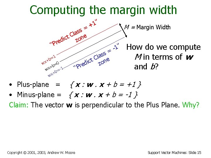
Computing the margin width ” 1 + = ss a l t C one c i z ed r P “ =1 b + 0 wx b= + wx b=-1 + wx M = Margin Width 1” = “P ss a l t C one c i z red How do we compute M in terms of w and b? • Plus-plane = { x : w. x + b = +1 } • Minus-plane = { x : w. x + b = -1 } Claim: The vector w is perpendicular to the Plus Plane. Why? Copyright © 2001, 2003, Andrew W. Moore Support Vector Machines: Slide 15

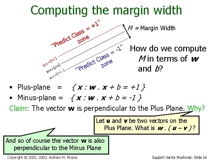
Computing the margin width ” 1 + = ss a l t C one c i z ed r P “ =1 b + 0 wx b= + wx b=-1 + wx M = Margin Width 1” = ss a l t C one c i z red “P How do we compute M in terms of w and b? • Plus-plane = { x : w. x + b = +1 } • Minus-plane = { x : w. x + b = -1 } Claim: The vector w is perpendicular to the Plus Plane. Why? Let u and v be two vectors on the Plus Plane. What is w. ( u – v ) ? And so of course the vector w is also perpendicular to the Minus Plane Copyright © 2001, 2003, Andrew W. Moore Support Vector Machines: Slide 16

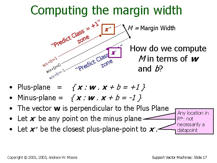
Computing the margin width 1” + + M = Margin Width = x s s la e C ct zon i d e “Pr 1” How do we compute x = s s la M in terms of w =1 C b e t + wx dic zon =0 e b r + and b? “P -1 wx = +b x w • • • Plus-plane = { x : w. x + b = +1 } Minus-plane = { x : w. x + b = -1 } The vector w is perpendicular to the Plus Plane Let x- be any point on the minus plane Let x+ be the closest plus-plane-point to x-. Copyright © 2001, 2003, Andrew W. Moore Any location in mm: : not � R not necessarily a datapoint Support Vector Machines: Slide 17

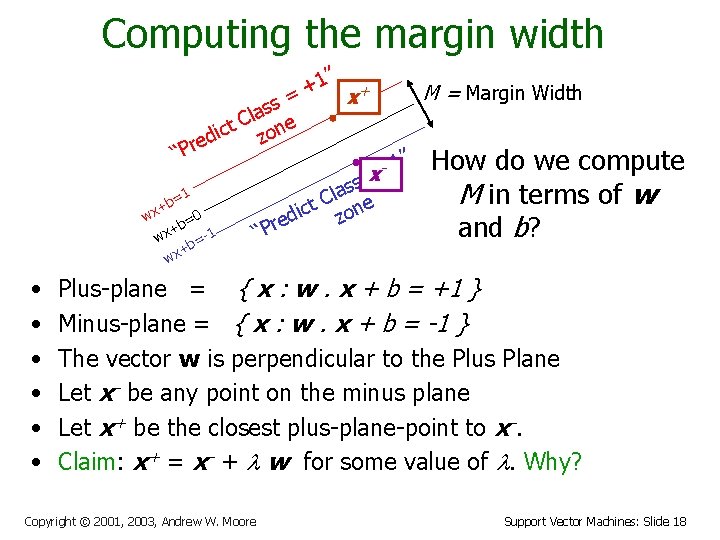
Computing the margin width 1” + + M = Margin Width = x s s la e C ct zon i d e “Pr 1” How do we compute x = s s la M in terms of w =1 C b e t + wx dic zon =0 e b r + and b? “P -1 wx = +b x w • • • Plus-plane = { x : w. x + b = +1 } Minus-plane = { x : w. x + b = -1 } The vector w is perpendicular to the Plus Plane Let x- be any point on the minus plane Let x+ be the closest plus-plane-point to x-. Claim: x+ = x- + l w for some value of l. Why? Copyright © 2001, 2003, Andrew W. Moore Support Vector Machines: Slide 18

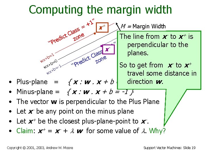
Computing the margin width 1” + + M = Margin Width = x s s la e C - to x+ is t n c The line from x i o z ed r P “ perpendicular to the do we compute 1” How x = s s planes. a 1 l M in terms of w = C b e t + wx dic zon =0 e b - to x+ r + P and b ? So to get from x 1 “ wx = wx • • • +b travel some distance in direction w. { x : w. x + b = +1 } Plus-plane = Minus-plane = { x : w. x + b = -1 } The vector w is perpendicular to the Plus Plane Let x- be any point on the minus plane Let x+ be the closest plus-plane-point to x-. Claim: x+ = x- + l w for some value of l. Why? Copyright © 2001, 2003, Andrew W. Moore Support Vector Machines: Slide 19

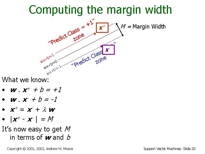
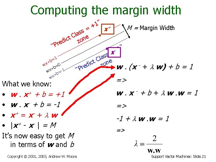
Computing the margin width 1” + + M = Margin Width = x s s la e C ct zon i d e “Pr 1” x = s s la =1 C b e t + c n i 0 o wx d z = re +b -1 P x “ w = +b x w What we know: • w. x+ + b = +1 • w. x- + b = -1 • x+ = x- + l w • |x + - x - | = M It’s now easy to get M in terms of w and b Copyright © 2001, 2003, Andrew W. Moore Support Vector Machines: Slide 20

Computing the margin width 1” + + M = Margin Width = x s s la e C ct zon i d e “Pr 1” x = s s la =1 C b e t + c n i 0 o wx d - + l w) + b z = re w. (x +b -1 P x “ w = +b x w What we know: • w. x+ + b = +1 • w. x- + b = -1 • x+ = x- + l w • |x + - x - | = M It’s now easy to get M in terms of w and b Copyright © 2001, 2003, Andrew W. Moore =1 => w. x - + b + l w. w = 1 => -1 + l w. w = 1 => Support Vector Machines: Slide 21

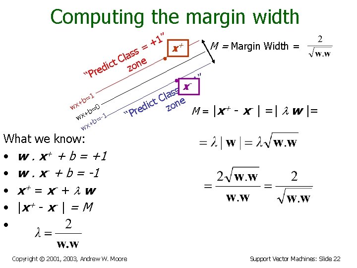
Computing the margin width 1” + + M = Margin Width = = x s s la e C ct zon i d e “Pr 1” x = s s la =1 C b e t + c n i 0 o wx d z = re M = |x+ - x- | =| l w |= +b -1 P x “ w = +b x w What we know: • w. x+ + b = +1 • w. x- + b = -1 • x+ = x- + l w • |x + - x - | = M • Copyright © 2001, 2003, Andrew W. Moore Support Vector Machines: Slide 22

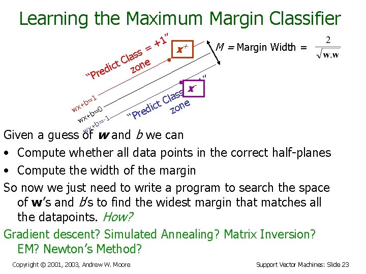
Learning the Maximum Margin Classifier 1” + + M = Margin Width = = x s s la e C ct zon i d e “Pr 1” x = s s la =1 C b e t + c n i 0 o wx d z = re +b -1 P x “ w = +b x w Given a guess of w and b we can • Compute whether all data points in the correct half-planes • Compute the width of the margin So now we just need to write a program to search the space of w’s and b’s to find the widest margin that matches all the datapoints. How? Gradient descent? Simulated Annealing? Matrix Inversion? EM? Newton’s Method? Copyright © 2001, 2003, Andrew W. Moore Support Vector Machines: Slide 23

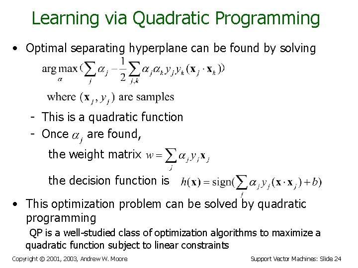
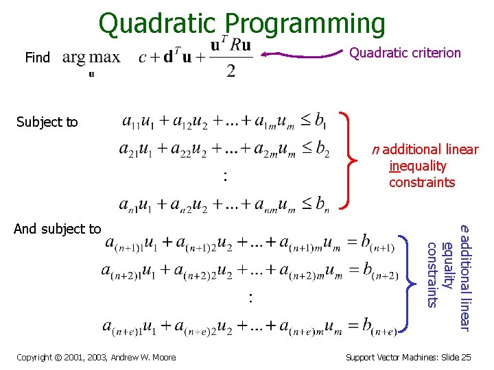
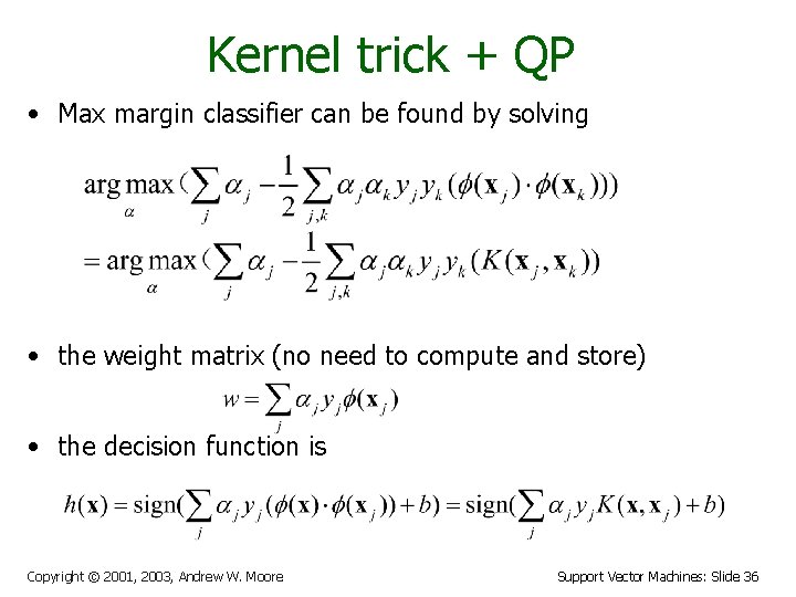
Learning via Quadratic Programming • Optimal separating hyperplane can be found by solving - This is a quadratic function - Once are found, the weight matrix the decision function is • This optimization problem can be solved by quadratic programming QP is a well-studied class of optimization algorithms to maximize a quadratic function subject to linear constraints Copyright © 2001, 2003, Andrew W. Moore Support Vector Machines: Slide 24

Quadratic Programming Find Quadratic criterion Subject to n additional linear inequality constraints Copyright © 2001, 2003, Andrew W. Moore e additional linear equality constraints And subject to Support Vector Machines: Slide 25

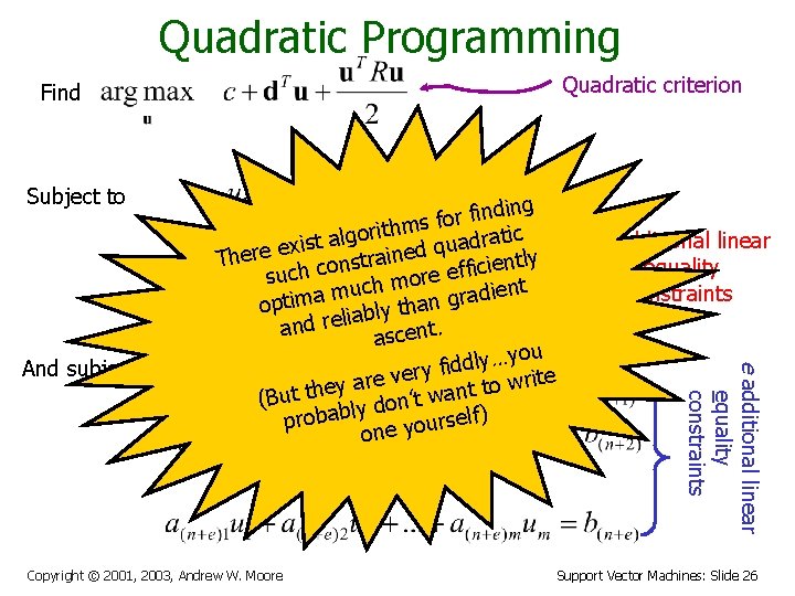
Quadratic Programming Quadratic criterion Find Subject to Copyright © 2001, 2003, Andrew W. Moore n additional linear inequality constraints e additional linear equality constraints And subject to ding n i f r o f thms i r o g l a ratic d t a s i u x q e ned i a There r t s ently n i o c i c f f h e c su more h c u ent i m d a a r m g i t op than y l b a i l and re ascent. you … y l d d i ery f v ite e r r w a o y t e t (But th ly don’t wan elf) s r probab u o y one Support Vector Machines: Slide 26

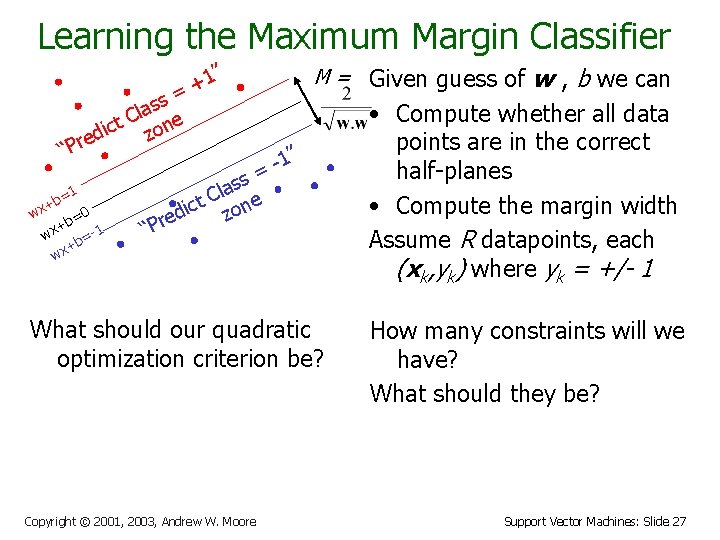
Learning the Maximum Margin Classifier ” M = Given guess of 1 + = “P +b =1 wx ss a l t C one c i z red 0 b= + wx b=-1 + wx 1” = ss a l t C one c i z ed r P “ What should our quadratic optimization criterion be? Copyright © 2001, 2003, Andrew W. Moore w , b we can • Compute whether all data points are in the correct half-planes • Compute the margin width Assume R datapoints, each (xk, yk) where yk = +/- 1 How many constraints will we have? What should they be? Support Vector Machines: Slide 27

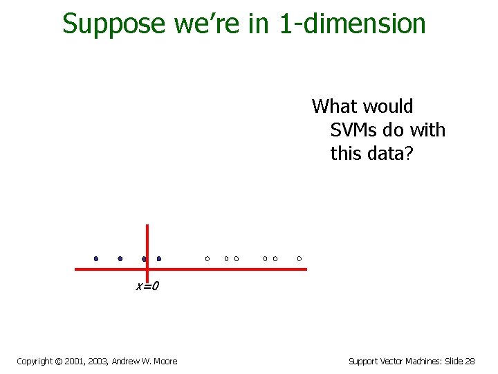
Suppose we’re in 1 -dimension What would SVMs do with this data? x=0 Copyright © 2001, 2003, Andrew W. Moore Support Vector Machines: Slide 28

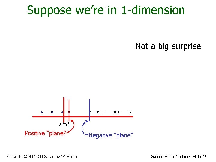
Suppose we’re in 1 -dimension Not a big surprise x=0 Positive “plane” Copyright © 2001, 2003, Andrew W. Moore Negative “plane” Support Vector Machines: Slide 29

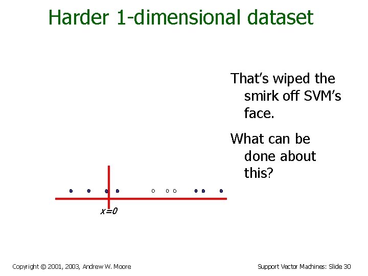
Harder 1 -dimensional dataset That’s wiped the smirk off SVM’s face. What can be done about this? x=0 Copyright © 2001, 2003, Andrew W. Moore Support Vector Machines: Slide 30

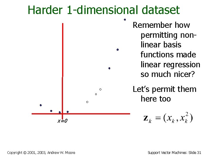
Harder 1 -dimensional dataset Remember how permitting nonlinear basis functions made linear regression so much nicer? Let’s permit them here too x=0 Copyright © 2001, 2003, Andrew W. Moore Support Vector Machines: Slide 31

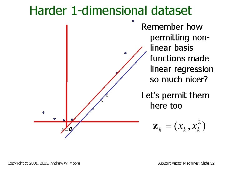
Harder 1 -dimensional dataset Remember how permitting nonlinear basis functions made linear regression so much nicer? Let’s permit them here too x=0 Copyright © 2001, 2003, Andrew W. Moore Support Vector Machines: Slide 32

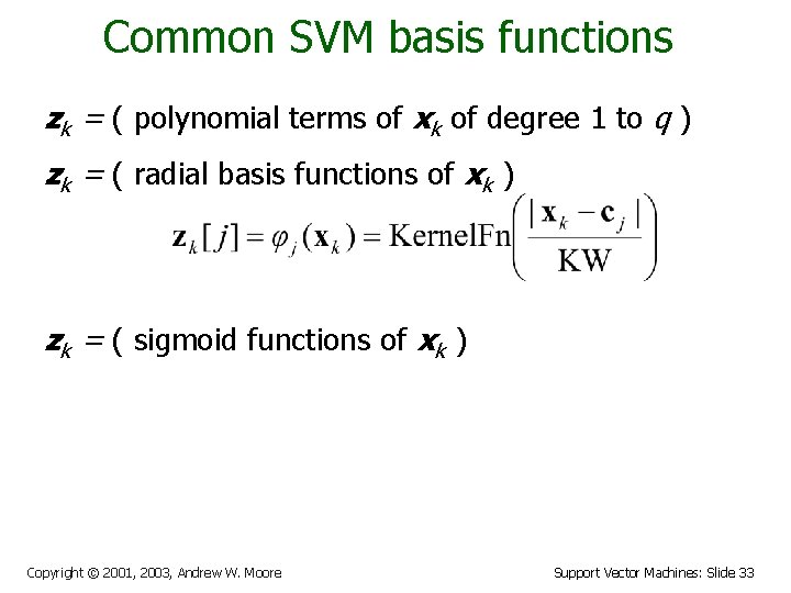
Common SVM basis functions zk = ( polynomial terms of xk of degree 1 to q ) zk = ( radial basis functions of xk ) zk = ( sigmoid functions of xk ) Copyright © 2001, 2003, Andrew W. Moore Support Vector Machines: Slide 33

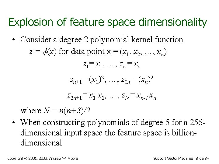
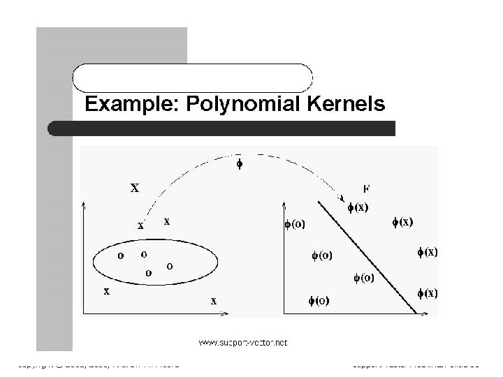
Explosion of feature space dimensionality • Consider a degree 2 polynomial kernel function z = (x) for data point x = (x 1, x 2, …, xn) z 1= x 1, …, zn = xn zn+1= (x 1)2, …, z 2 n = (xn)2 z 2 n+1= x 1, …, z. N = xn-1 xn where N = n(n+3)/2 • When constructing polynomials of degree 5 for a 256 dimensional input space the feature space is billiondimensional Copyright © 2001, 2003, Andrew W. Moore Support Vector Machines: Slide 34

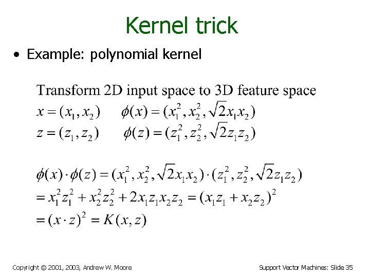
Kernel trick • Example: polynomial kernel Copyright © 2001, 2003, Andrew W. Moore Support Vector Machines: Slide 35

Kernel trick + QP • Max margin classifier can be found by solving • the weight matrix (no need to compute and store) • the decision function is Copyright © 2001, 2003, Andrew W. Moore Support Vector Machines: Slide 36

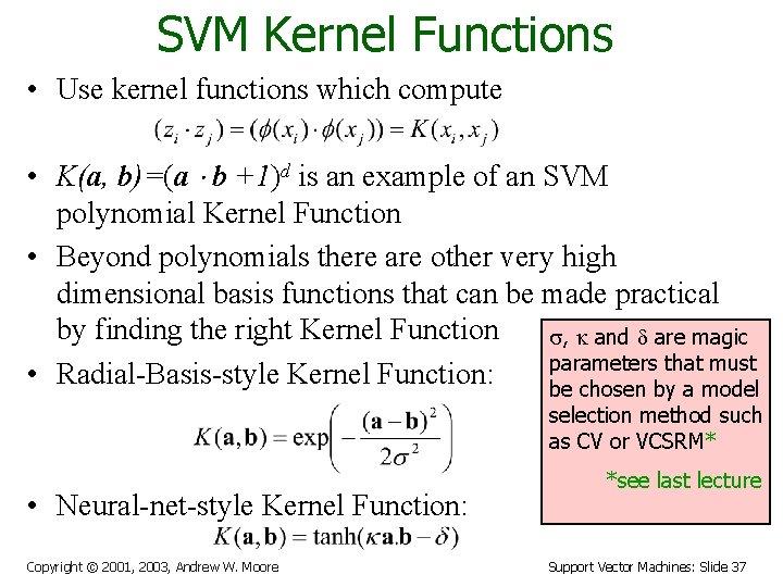
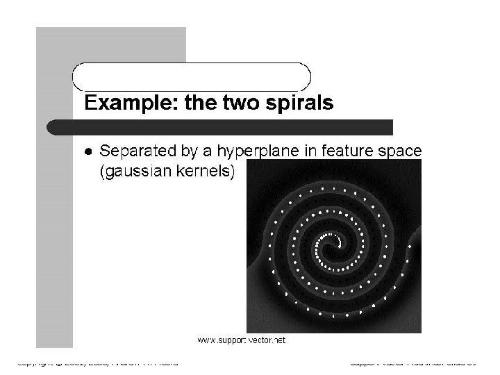
SVM Kernel Functions • Use kernel functions which compute • K(a, b)=(a b +1)d is an example of an SVM polynomial Kernel Function • Beyond polynomials there are other very high dimensional basis functions that can be made practical by finding the right Kernel Function s, k and d are magic parameters that must • Radial-Basis-style Kernel Function: be chosen by a model selection method such as CV or VCSRM* • Neural-net-style Kernel Function: Copyright © 2001, 2003, Andrew W. Moore *see last lecture Support Vector Machines: Slide 37

Copyright © 2001, 2003, Andrew W. Moore Support Vector Machines: Slide 38

Copyright © 2001, 2003, Andrew W. Moore Support Vector Machines: Slide 39

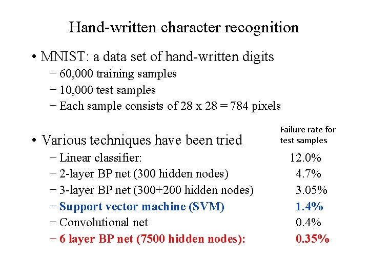
SVM Performance • Anecdotally they work very well indeed. • Overcomes linear separability problem • Transforming input space to a higher dimension feature space • Overcome dimensionality explosion by kernel trick • Generalizes well (overfitting not as serious) • Maximum margin separator • Find MMS by quadratic programming • Example: • currently the best-known classifier on a well-studied handwritten-character recognition benchmark • several reliable people doing practical real-world work claim that SVMs have saved them when their other favorite classifiers did poorly. Copyright © 2001, 2003, Andrew W. Moore Support Vector Machines: Slide 40

Hand-written character recognition • MNIST: a data set of hand-written digits − 60, 000 training samples − 10, 000 test samples − Each sample consists of 28 x 28 = 784 pixels • Various techniques have been tried − Linear classifier: − 2 -layer BP net (300 hidden nodes) − 3 -layer BP net (300+200 hidden nodes) − Support vector machine (SVM) − Convolutional net − 6 layer BP net (7500 hidden nodes): Failure rate for test samples 12. 0% 4. 7% 3. 05% 1. 4% 0. 35%

SVM Performance • There is a lot of excitement and religious fervor about SVMs as of 2001. • Despite this, some practitioners are a little skeptical. Copyright © 2001, 2003, Andrew W. Moore Support Vector Machines: Slide 42

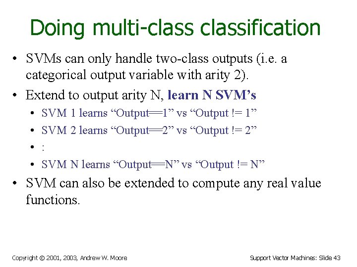
Doing multi-classification • SVMs can only handle two-class outputs (i. e. a categorical output variable with arity 2). • Extend to output arity N, learn N SVM’s • • SVM 1 learns “Output==1” vs “Output != 1” SVM 2 learns “Output==2” vs “Output != 2” : SVM N learns “Output==N” vs “Output != N” • SVM can also be extended to compute any real value functions. Copyright © 2001, 2003, Andrew W. Moore Support Vector Machines: Slide 43

References • An excellent tutorial on VC-dimension and Support Vector Machines: C. J. C. Burges. A tutorial on support vector machines for pattern recognition. Data Mining and Knowledge Discovery, 2(2): 955 -974, 1998. http: //citeseer. nj. nec. com/burges 98 tutorial. html • The VC/SRM/SVM Bible: Statistical Learning Theory by Vladimir Vapnik, Wiley. Interscience; 1998 • Download SVM-light: http: //svmlight. joachims. org/ Copyright © 2001, 2003, Andrew W. Moore Support Vector Machines: Slide 44