Digital Image Processing Image Compression Caution The PDF

Digital Image Processing Image Compression Caution: The PDF version of this presentation will appear to have errors due to heavy use of animations Material in this presentation is largely based on/derived from presentation(s) and book: The Digital Image by Dr. Donald House at Texas A&M University Brent M. Dingle, Ph. D. Game Design and Development Program Mathematics, Statistics and Computer Science University of Wisconsin - Stout 2015

Lecture Objectives • Previously – Filtering – Interpolation – Warping – Morphing Image Manipulation and Enhancement • Today – Image Compression

Definition: File Compression • Compression: the process of encoding information in fewer bits – Wasting space is bad, so compression is good – Image Compression • Redundant information in images – Identical colors – Smooth variation in light intensity – Repeating texture

Identical Colors Mondrian’s Composition 1930

Smooth Variation in Light Intensity Digital rendering using Autodesk VIZ. (Image Credit: Alejandro Vazquez. )

Repeating Texture Alvar Aalto Summer House 1953

What is Compression Really? • Works because of data redundancy – Temporal • In 1 D data, 1 D signals, Audio… – Spatial • correlation between neighboring pixels or data items – Spectral • correlation between color or luminescence components • uses the frequency domain to exploit relationships between frequency of change in data – Psycho-visual • exploits perceptual properties of the human (visual) system

Two General Types • Lossless Compression – data is compressed and can be uncompressed without loss of detail or information • bit-preserving • reversible • Lossy Compression – purpose is to obtain the best possible fidelity for a given bit-rate • or minimizing the bit-rate to achieve a given fidelity measure – Video and audio commonly use lossy compression • because humans have limited perception of finer details

Two Types • Lossless compression often involves some form of entropy encoding – based in information theoretic techniques • see next slide for visual • Lossy compression uses source encoding techniques that may involve transform encoding, differential encoding or vector quanatization • see next slide for visual

Compression Methods

Compression Methods next up

Simple Lossless Compression • Simple Repetition Suppression – If a sequence contains a series of N successive tokens – Then they can be replaced with a single token and a count of the number of times the token repeats • This does require a flag to denote when the repeated token appears – Example • • 12344444 can be denoted 123 f 9 where f is the flag for four

Run-length Encoding (RLE) • RLE is often applied to images – It is a small component used in JPEG compression • Conceptually – sequences of image elements X 1, X 2, …, Xn are mapped to pairs (c 1, L 1), (c 2, L 2), …, (cn, Ln) • where ci represent the image intensity or color • and Li the length of the ith run of pixels

Run-Length Encoding (RLE): lossless • Scanline: 2 2 2 2 3 4 1 1 1 • Run-length encoding ( 7 2) (1 3) (1 4) (3 1) 12 values 8 values

Run-Length Encoding (RLE): lossless • Scanline: 2 2 2 2 3 4 1 12 values run of repeating values • Run-length encoding ( 7 2) (1 3) (1 4) (3 1) repeat count 8 values pixel value 25% reduction of memory use

RLE: worst case • Scanline: 1 2 3 4 5 6 7 8 • Run-length encoding: (1 1)(1 2)(1 3)(1 4)(1 5)(1 6)(1 7) 8 values 16 values doubles space

RLE: Improving • Scanline: 5 5 5 5 3 4 1 1 1 • Run-length encoding need to flag this as meaning “not repeating” ( 7 5) (2 3 4)(3 1) (7 2) 5 5 5 5 (2 3 4) 3 4 (3 1) 1 1 1 the flag indicates that 2 explicitly given values follow Using this improvement The worst case then only adds 1 extra value

How to flag the repeat/no repeat? • SGI Iris RGB Run-length Encoding Scheme

Compression Methods next up

Compression: Pattern Substitution • Pattern Substitution, lossless • Simple form of statistical encoding • Concept – Substitute a frequently repeating pattern with a shorter code • the shorter code(s) may be predefined by the algorithm being used or dynamically created

Table Lookup • Table Lookup can be viewed as a Pattern Substitution Method • Example – Allow full range of colors (24 bit, RGB) – Image only uses 256 (or less) unique colors (8 bits) – Create a table of which colors are used • Use 8 bits for each color instead of 24 bits – Conceptually how older BMPs worked » color depth <= 8 bits

Table Lookup: GIF • Graphics Interchange File Format (GIF) – uses table lookups Color Look. Up Table (CLUT)

GIF Compression with Color Look. Up Table (CLUT) Example Image Size = 1000 x 1000 256 colors Each color 24 bit (RGB) without CLUT 1000*24 bits with CLUT 1000*8 bit (index data) + 3*256*8 bit (table data) Use about 2/3 the space (when image size is “big”)

Compression: Pattern Substitution • Table lookups work • But Pattern Substitution typically is more dynamic – Counts occurrence of tokens – Sorts (say descending order) – Assign highest counts shortest codes

Compression Methods next up

Lossless Compression: Entropy Encoding • Lossless compression often involves some form of entropy encoding and are based in information theoretic techniques – Aside: • Claude Shannon is considered the father of information theory

Shannon-Fano Algorithm • Technique proposed in Shannon’s 1948 article. introducing the field of Information Theory: – A Mathematical Theory of Communication • Shannon, C. E. (July 1948). "A Mathematical Theory of Communication". Bell System Technical Journal 27: 379– 423. • Method Attributed to Robert Fano, as published in a technical report – The transmission of information • Fano, R. M. (1949). "The transmission of information". Technical Report No. 65 (Cambridge (Mass. ), USA: Research Laboratory of Electronics at MIT).

Example: Shannon-Fano Algorithm Symbol A B C D E Count 15 7 6 6 5

Example: Shannon-Fano Algorithm Symbol E B A D C Count 15 7 6 6 5 Step 1: Sort the symbols by frequency/probability As shown: E B A D C

Example: Shannon-Fano Algorithm Symbol E B A D C Count 15 7 6 6 5 Step 1: Sort the symbols by frequency/probability Step 2: Recursively divide into 2 parts Each with about same number of counts As shown: Dividing between B and A results in 22 on the left and 17 on the right -- minimizing difference totals between groups This division means E and B codes start with 0 and A D and C codes start with 1 E B A D C

Example: Shannon-Fano Algorithm Symbol E B A D C Count 15 7 6 6 5 Step 1: Sort the symbols by frequency/probability Step 2: Recursively divide into 2 parts Each with about same number of counts As shown: Dividing between B and A results in 22 on the left and 17 on the right -- minimizing difference totals between groups E B A D C This division means E and B codes start with 0 and A D and C codes start with 1 E and B are then divided (15: 7) A is divided from D and C (6: 11) So E is leaf with code 00, B is a leaf with code 01 A is a leaf with code 10 D and C need divided again

Example: Shannon-Fano Algorithm Symbol E B A D C Count 15 7 6 6 5 Step 1: Sort the symbols by frequency/probability Step 2: Recursively divide into 2 parts Each with about same number of counts As shown: So E is leaf with code 00, B is a leaf with code 01 A is a leaf with code 10 D and C need divided again Divide D and C (6: 5) E B A D C D becomes a leaf with code 110 C becomes a leaf with code 111

Example: Shannon-Fano Algorithm Symbol E B A D C Count 15 7 6 6 5 Step 1: Sort the symbols by frequency/probability Step 2: Recursively divide into 2 parts Each with about same number of counts As shown: Final Encoding: Symbol E B A D C Count 00 01 10 111 E B A D C

Compression Methods next up

Quick Summary: Huffman Algorithm • Encoding Summary Step 1: Initialization Put all nodes in an OPEN list (keep it sorted at all times) Step 2: While OPEN list has more than 1 node Step 2 a: From OPEN pick 2 nodes having the lowest frequency/probability Create a parent node for them Step 2 b: Assign the sum of the frequencies of the selected node to their newly created parent Step 2 c: Assign code 0 to the left branch Assign code 1 to the right branch Remove the selected children from OPEN (note the newly created parent node remains in OPEN)

Observation • Some characters in the English alphabet occur more frequently than others – The table below is based on Robert Lewand's Cryptological Mathematics

Huffman Encoding (English Letters) • Huffman encoding: Uses variable lengths for different characters to take advantage of their relative frequencies – Some characters occur more often than others • If those characters use < 8 bits each, the file will be smaller – Other characters may need > 8 bits • but that’s ok they don’t show up often

Huffman’s Algorithm • The idea: Create a “Huffman Tree” that will tell us a good binary representation for each character – Left means 0 – Right means 1 • Example 'b‘ is 10 • More frequent characters will be higher in the tree (have a shorter binary value). • To build this tree, we must do a few steps first – Count occurrences of each unique character in the file to compress – Use a priority queue to order them from least to most frequent – Make a tree and use it

Huffman Compression – Overview • Step 1 – Count characters (frequency of characters in the message) • Step 2 – Create a Priority Queue • Step 3 – Build a Huffman Tree • Step 4 – Traverse the Tree to find the Character to Binary Mapping • Step 5 – Use the mapping to encode the message

Step 1: Count Characters • Example message (input file) contents: file ends with an invisible EOF ab ab character – counts: { ' ' = 2, 'b'=3, 'a' =3, 'c' =1, EOF=1 } byte 1 2 3 4 5 6 7 8 9 10 char 'a' 'b' ' ' 'c' 'a' 'b' EOF ASCII 97 98 32 99 97 98 256 binary 01100001 011000100000 01100011 01100001 01100010 N/A – File size currently = 10 bytes = 80 bits

Step 2: Create a Priority Queue • Each node of the PQ is a tree – The root of the tree is the ‘key’ – The other internal nodes hold ‘subkeys’ – The leaves hold the character values • Insert each into the PQ using the PQ’s function – insert. Item(count, character) • The PQ should organize them into ascending order – So the smallest value is highest priority • We will use an example with the PQ implemented as an ordered list – But the PQ could be implemented in whatever way works best » could be a minheap, unordered list, or ‘other’

Step 2: PQ Creation, An Illustration • From step 1 we have – counts: { ' ' = 2, 'b'=3, 'a'=3, 'c'=1, EOF=1 } • Make these into trees • Add the trees to a Priority Queue – Assume PQ is implemented as a sorted list

Step 2: PQ Creation, An Illustration • From step 12 we 3 have 3 1 1 – counts: { ' ' = 2, 'b'=3, 'a'=3, 'c'=1, EOF=1 } • Make these ' 'intobtrees a c EOF • Add the trees to a Priority Queue – Assume PQ is implemented as a sorted list

Step 2: PQ Creation, An Illustration • From step 1 we have – counts: { ' ' = 2, 'b'=3, 'a'=3, 'c'=1, EOF=1 } • Make these into trees • Add the trees to a Priority Queue – Assume PQ is implemented as a sorted list eration rt is an O(n) op 2 se In h ac E l: al ) Rec. So this is O(n es m ti n e on d This is 3123 EOF 'acb'

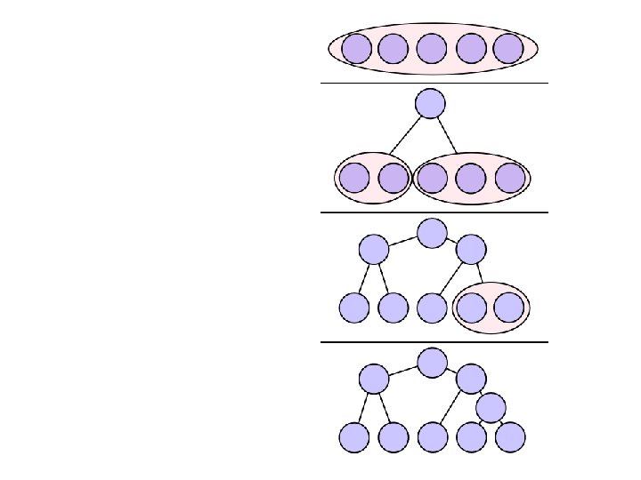
Step 3: Build the Huffman Tree • Aside: All nodes should be in the PQ • While PQ. size() > 1 – Remove the two highest priority (rarest) nodes • Removal done using PQ’s remove. Min() function – Combine the two nodes into a single node • So the new node is a tree with – root has key value = sum of keys of nodes being combined – left subtree is the first removed node – right subtree is the second removed node – Insert the combined node back into the PQ • end While • Remove the one node from the PQ – This is the Huffman Tree ple m Exa e ne lid s t x

Step 3 a: Building Huffman Tree, Illus. • Remove the two highest priority (rarest) nodes 1 1 2 3 3 c EOF ' ' b a

Step 3 b: Building Huffman Tree, Illus. • Combine the two nodes into a single node 2 1 1 c EOF 2 3 3 ' ' b a

Step 3 c: Building Huffman Tree, Illus. • Insert the combined node back into the PQ 2 1 1 c EOF 2 3 3 ' ' b a

Step 3 d: Building Huffman Tree, Illus. • PQ has 4 nodes still, so repeat 2 2 ' ' 1 1 c EOF 3 3 b a

Step 3 a: Building Huffman Tree, Illus. • Remove the two highest priority (rarest) nodes 2 2 ' ' 1 1 c EOF 3 3 b a

Step 3 b: Building Huffman Tree, Illus. • Combine the two nodes into a single node 4 2 2 ' ' 1 1 c EOF 3 3 b a

Step 3 c: Building Huffman Tree, Illus. • Insert the combined node back into the PQ 4 2 2 ' ' 1 1 c EOF 3 3 b a

Step 3 d: Building Huffman Tree, Illus. • 3 nodes remain in PQ, repeat again 3 3 b a 4 2 2 ' ' 1 1 c EOF

Step 3 a: Building Huffman Tree, Illus. • Remove the two highest priority (rarest) nodes 3 3 b a 4 2 2 ' ' 1 1 c EOF

Step 3 b: Building Huffman Tree, Illus. • Combine the two nodes into a single node 4 6 2 2 3 3 b a ' ' 1 1 c EOF

Step 3 c: Building Huffman Tree, Illus. • Insert the combined node back into the PQ 4 6 2 2 3 3 b a ' ' 1 1 c EOF

Step 3 d: Building Huffman Tree, Illus. • 2 nodes still in PQ, repeat one more time 4 6 2 2 ' ' 1 1 c EOF 3 3 b a

Step 3 a: Building Huffman Tree, Illus. • Remove the two highest priority (rarest) nodes 4 6 2 2 ' ' 1 1 c EOF 3 3 b a

Step 3 b: Building Huffman Tree, Illus. • Combine the two nodes into a single node 10 4 6 2 2 ' ' 1 1 c EOF 3 3 b a

Step 3 c: Building Huffman Tree, Illus. • Insert the combined node back into the PQ 10 4 6 2 2 ' ' 1 1 c EOF 3 3 b a

Step 3 d: Building Huffman Tree, Illus. • Only 1 node remains in the PQ, so while loop ends 10 4 6 2 2 ' ' 1 1 c EOF 3 3 b a

Step 3: Building Huffman Tree, Illus. • Huffman tree is complete 10 4 6 2 2 ' ' 1 1 c EOF 3 3 b a

Step 4: Traverse Tree to Find the Character to Binary Mapping • • • ' ' 'c' EOF 'b' 'a' = = = Recall Left is 0 Right is 1 10 4 6 2 2 ' ' 1 1 c EOF 3 3 b a

Step 4: Traverse Tree to Find the Character to Binary Mapping • • • ' ' 'c' EOF 'b' 'a' = = = 00 Recall Left is 0 Right is 1 10 0 4 6 0 2 2 ' ' 1 1 c EOF 3 3 b a

Step 4: Traverse Tree to Find the Character to Binary Mapping • • • ' ' 'c' EOF 'b' 'a' = = = 00 010 Recall Left is 0 Right is 1 10 0 4 6 1 2 2 ' ' 0 1 1 c EOF 3 3 b a

Step 4: Traverse Tree to Find the Character to Binary Mapping • • • ' ' 'c' EOF 'b' 'a' = = = 00 011 Recall Left is 0 Right is 1 10 0 4 6 1 2 2 1 ' ' 1 1 c EOF 3 3 b a

Step 4: Traverse Tree to Find the Character to Binary Mapping • • • ' ' 'c' EOF 'b' 'a' = = = 00 010 10 011 Recall Left is 0 Right is 1 1 10 4 6 0 2 2 ' ' 1 1 c EOF 3 3 b a

Step 4: Traverse Tree to Find the Character to Binary Mapping • • • ' ' 'c' EOF 'b' 'a' = = = 00 010 10 011 Recall Left is 0 Right is 1 1 10 11 4 6 1 2 2 ' ' 1 1 c EOF 3 3 b a

Step 5: Encode the Message • • • ' ' 'c' EOF 'b' 'a' • = 00 = 011 = 10 = 11 Example message (input file) contents: ab ab cab 10 4 6 2 2 ' ' 1 1 c EOF 3 3 b a file ends with an invisible EOF character

Challenge: Encode the Message • • • ' ' 'c' EOF 'b' 'a' = 00 = 011 = 10 = 11 • Example message (input file) contents: ab ab cab file ends with an invisible EOF character

Step 5: Encode the Message • • • ' ' 'c' EOF 'b' 'a' = 00 = 011 = 10 = 11 • Example message (input file) contents: ab ab cab file ends with an invisible EOF character

Step 5: Encode the Message • • • ' ' 'c' EOF 'b' 'a' = 00 = 011 = 10 = 11 • 1110 • Example message (input file) contents: ab ab cab file ends with an invisible EOF character

Step 5: Encode the Message • • • ' ' 'c' EOF 'b' 'a' = 00 = 011 = 10 = 11 • 111000 • Example message (input file) contents: ab ab cab file ends with an invisible EOF character

Step 5: Encode the Message • • • ' ' 'c' EOF 'b' 'a' = 00 = 011 = 10 = 11 • 11100011 • Example message (input file) contents: ab ab cab file ends with an invisible EOF character

Step 5: Encode the Message • • • ' ' 'c' EOF 'b' 'a' = 00 = 011 = 10 = 11 • Example message (input file) contents: • 1110001110 ab ab cab file ends with an invisible EOF character

Step 5: Encode the Message • • • ' ' 'c' EOF 'b' 'a' = 00 = 011 = 10 = 11 • Example message (input file) contents: ab ab cab • 111000 file ends with an invisible EOF character

Step 5: Encode the Message • • • ' ' 'c' EOF 'b' 'a' = 00 = 011 = 10 = 11 • Example message (input file) contents: ab ab cab • 111000010 file ends with an invisible EOF character

Step 5: Encode the Message • • • ' ' 'c' EOF 'b' 'a' = 00 = 011 = 10 = 11 • Example message (input file) contents: ab ab cab • 11100001011 file ends with an invisible EOF character

Step 5: Encode the Message • • • ' ' 'c' EOF 'b' 'a' = 00 = 011 = 10 = 11 • Example message (input file) contents: ab ab cab • 1110000101110 file ends with an invisible EOF character

Step 5: Encode the Message • • • ' ' 'c' EOF 'b' 'a' = 00 = 011 = 10 = 11 • Example message (input file) contents: ab ab cab • 1110000101110011 file ends with an invisible EOF character

Step 5: Encode the Message • • • ' ' 'c' EOF 'b' 'a' = 00 = 011 = 10 = 11 • Example message (input file) contents: ab ab cab • 1110000101110011 • Count the bits used = 22 bits • versus the 80 • previously needed • File is almost ¼ the size • lots of savings file ends with an invisible EOF character

Decompression • From the previous tree shown we now have the message characters encoded as: char 'a' 'b' ' ' 'c' 'a' 'b' EOF binary 11 10 00 010 11 10 011 • Which compresses to bytes 3 like so: 1 byte char a b 2 a binary 11 10 00 11 b c 3 a b EOF 10 00 010 1 1 10 011 • How to decompress? • Hint: Lookup table is not the best answer, what is the first symbol? . . . 1=? or is it 11? or 1110? or…

Decompression via Tree • The tree is known to the recipient of the message • So use it • To identify symbols we will Apply the Prefix Property • No encoding A is the prefix of another encoding B • Never will have x 011 and y 011100110

Decompression via Tree • Apply the Prefix Property • No encoding A is the prefix of another encoding B • Never will have x 011 and y 011100110 • the Algorithm • • Read each bit one at a time from the input If the bit is 0 go left in the tree Else if the bit is 1 go right If you reach a leaf node • output the character at that leaf • and go back to the tree root

Decompressing Example • Say the encrypted message was: 10 • 10110100011011 • note: this is NOT the same message as the encryption just done (but the tree the is same) 4 6 • Read each bit one at a time • If it is 0 go left • If it is 1 go right • If you reach a leaf, output the character there and go back to the tree root 2 2 ' ' 1 1 c EOF 3 3 b a

Class Activity: Decompressing Example • Say the encrypted message was: 10 • 10110100011011 • note: this is NOT the same message as the encryption just done (but the tree the is same) 4 6 • Read each bit one at a time • If it is 0 go left • If it is 1 go right • If you reach a leaf, output the character there and go back to the tree root • Pause for students to complete 2 2 ' ' 1 1 c EOF 3 3 b a

Decompressing Example • Say the encrypted message was: 10 • 10110100011011 1 4 6 • Read each bit one at a time • If it is 0 go left • If it is 1 go right • If you reach a leaf, output the character there and go back to the tree root 2 2 ' ' 1 1 c EOF 3 3 b a

Decompressing Example • Say the encrypted message was: 10 • 10110100011011 1 b 4 6 0 • Read each bit one at a time • If it is 0 go left • If it is 1 go right • If you reach a leaf, output the character there and go back to the tree root 2 2 ' ' 1 1 c EOF 3 3 b a

Decompressing Example • Say the encrypted message was: 10 • 10110100011011 1 b 4 6 • Read each bit one at a time • If it is 0 go left • If it is 1 go right • If you reach a leaf, output the character there and go back to the tree root 2 2 ' ' 1 1 c EOF 3 3 b a

Decompressing Example • Say the encrypted message was: 10 • 10110100011011 1 b a 4 6 1 • Read each bit one at a time • If it is 0 go left • If it is 1 go right • If you reach a leaf, output the character there and go back to the tree root 2 2 ' ' 1 1 c EOF 3 3 b a

Decompressing Example • Say the encrypted message was: 10 • 10110100011011 0 b a 4 6 • Read each bit one at a time • If it is 0 go left • If it is 1 go right • If you reach a leaf, output the character there and go back to the tree root 2 2 ' ' 1 1 c EOF 3 3 b a

Decompressing Example • Say the encrypted message was: 10 • 10110100011011 0 b a 4 1 • Read each bit one at a time • If it is 0 go left • If it is 1 go right • If you reach a leaf, output the character there and go back to the tree root 6 2 2 ' ' 1 1 c EOF 3 3 b a

Decompressing Example • Say the encrypted message was: 10 • 10110100011011 0 b a c 4 1 • Read each bit one at a time • If it is 0 go left • If it is 1 go right • If you reach a leaf, output the character there and go back to the tree root 6 2 2 0 ' ' 1 1 c EOF 3 3 b a

Decompressing Example • Say the encrypted message was: 10 • 10110100011011 b a c 0 4 6 • Read each bit one at a time • If it is 0 go left • If it is 1 go right • If you reach a leaf, output the character there and go back to the tree root 2 2 ' ' 1 1 c EOF 3 3 b a

Decompressing Example • Say the encrypted message was: 10 • 10110100011011 b a c 4 • If you reach a leaf, output the character there and go back to the tree root 6 0 • Read each bit one at a time • If it is 0 go left • If it is 1 go right 0 2 2 ' ' 1 1 c EOF 3 3 b a

Decompressing Example • Say the encrypted message was: 10 • 10110100011011 1 b a c 4 6 • Read each bit one at a time • If it is 0 go left • If it is 1 go right • If you reach a leaf, output the character there and go back to the tree root 2 2 ' ' 1 1 c EOF 3 3 b a

Decompressing Example • Say the encrypted message was: 10 • 10110100011011 b a c 1 a 4 6 1 • Read each bit one at a time • If it is 0 go left • If it is 1 go right • If you reach a leaf, output the character there and go back to the tree root 2 2 ' ' 1 1 c EOF 3 3 b a

Decompressing Example • Say the encrypted message was: 10 • 10110100011011 b a c 0 a 4 6 • Read each bit one at a time • If it is 0 go left • If it is 1 go right • If you reach a leaf, output the character there and go back to the tree root 2 2 ' ' 1 1 c EOF 3 3 b a

Decompressing Example • Say the encrypted message was: 10 • 10110100011011 b a c 0 a 4 1 • Read each bit one at a time • If it is 0 go left • If it is 1 go right • If you reach a leaf, output the character there and go back to the tree root 6 2 2 ' ' 1 1 c EOF 3 3 b a

Decompressing Example • Say the encrypted message was: 10 • 10110100011011 b a c 0 a c 4 1 • Read each bit one at a time • If it is 0 go left • If it is 1 go right • If you reach a leaf, output the character there and go back to the tree root 6 2 2 0 ' ' 1 1 c EOF 3 3 b a

Decompressing Example • Say the encrypted message was: 10 • 10110100011011 b a c 1 a c 4 6 • Read each bit one at a time • If it is 0 go left • If it is 1 go right • If you reach a leaf, output the character there and go back to the tree root 2 2 ' ' 1 1 c EOF 3 3 b a

Decompressing Example • Say the encrypted message was: 10 • 10110100011011 b a c 1 a c a 4 6 1 • Read each bit one at a time • If it is 0 go left • If it is 1 go right • If you reach a leaf, output the character there and go back to the tree root 2 2 ' ' 1 1 c EOF 3 3 b a

Decompressing Example • Say the encrypted message was: 10 • 10110100011011 b a c 0 a c a 4 6 • Read each bit one at a time • If it is 0 go left • If it is 1 go right • If you reach a leaf, output the character there and go back to the tree root 2 2 ' ' 1 1 c EOF 3 3 b a

Decompressing Example • Say the encrypted message was: 10 • 10110100011011 b a c 0 a c a 4 1 • Read each bit one at a time • If it is 0 go left • If it is 1 go right • If you reach a leaf, output the character there and go back to the tree root 6 2 2 ' ' 1 1 c EOF 3 3 b a

Decompressing Example • Say the encrypted message was: 10 • 10110100011011 b a c a 0 EOF 4 1 • Read each bit one at a time • If it is 0 go left • If it is 1 go right • If you reach a leaf, output the character there and go back to the tree root 6 2 2 1 ' ' 1 1 c EOF 3 3 b a

Decompressing Example • Say the encrypted message was: 10 • 10110100011011 b a c a EOF d de o c e d w o n s i e l i f And the 4 6 • Read each bit one at a time • If it is 0 go left • If it is 1 go right • If you reach a leaf, output the character there and go back to the tree root 2 2 ' ' 1 1 c EOF 3 3 b a

Compression Methods up next: ONE MORE EXAMPLE

Lempel-Ziv-Welch (LZW) Compression • Lossless • Has a table • Does not store the table

LZW Compression • Discovers and remembers patterns of colors • Stores the patterns in a table – BUT only table indices are stored in the file • LZW table entries can grow arbitrarily long, – So one table index can stand for a long string of data in the file – BUT again the table itself never needs to be stored in the file

LZW Encoder: Pseudocode RGB = 3 bytes but idea stays same From Chapter 3 of MIT 6. 02 DRAFT Lecture Notes, Feb 13, 2012

LZW Decoder: Pseudocode RGB = 3 bytes but idea stays same ry From Chapter 3 of MIT 6. 02 DRAFT Lecture Notes, Feb 13, 2012

Questions? • Beyond D 2 L – Examples and information can be found online at: • http: //docdingle. com/teaching/cs. html • Continue to more stuff as needed

Extra Reference Stuff Follows

Credits • Much of the content derived/based on slides for use with the book: – Digital Image Processing, Gonzalez and Woods • Some layout and presentation style derived/based on presentations by – – – – Donald House, Texas A&M University, 1999 Bernd Girod, Stanford University, 2007 Shreekanth Mandayam, Rowan University, 2009 Igor Aizenberg, TAMUT, 2013 Xin Li, WVU, 2014 George Wolberg, City College of New York, 2015 Yao Wang and Zhu Liu, NYU-Poly, 2015 Sinisa Todorovic, Oregon State, 2015