Data Mining Basic Functionalities Chapter 2 MIS 214

Data Mining: Basic Functionalities — Chapter 2 — MIS 214 2014/2015 Spring 1

Chapter 2: Basic Data Mining Techniques n Decision Trees: ID 3 Algorithm n Association Rule Mining: Apriori Algorithm n Clustering: K-Means Algorıthm 2

Classification by Decision Tree Induction n Decision tree n A flow-chart-like tree structure n Internal node denotes a test on an attribute n Branch represents an outcome of the test n Leaf nodes represent class labels or class distribution Decision tree generation consists of two phases n Tree construction n At start, all the training examples are at the root n Partition examples recursively based on selected attributes n Tree pruning n Identify and remove branches that reflect noise or outliers Once the tree is build n Use of decision tree: Classifying an unknown sample 3

Training Dataset This follows an example from Quinlan’s ID 3 Han Table 7. 1 Original data from DMPML Ch 4 Sec 4. 3 pp 8 -9, 89 -94 4

In Practice passed Ii n n Current Oi time For the i th data, n at time I, input information is known n At time O, output is asigned (yes/no) For all data object in the training data set (i=1. . 14) both input and output are known 5

In Practice passed Current In n future On time For a new customers n, n at the current time I, input information is known n But O, output is not known Yet to be classified as (yes or no) before its actual buying behavioris realized Value of a data mining study to predict buying behavior beforehand 6

Output: A Decision Tree for “buys_computer” age? 5 cases <=30 student? 14 cases overcast 31. . 40 >40 5 cases yes credit rating? no yes excellent fair no yes 7
")
ID 3 Algorithm for Decision Tree Induction n n ID 3 algorithm Quinlan (1986) n Tree is constructed in a top-down recursive divide-and-conquer manner n At start, all the training examples are at the root n Attributes are categorical (if continuous-valued, they are discretized in advance) n Examples are partitioned recursively based on selected attributes n Test attributes are selected on the basis of a heuristic or statistical measure (e. g. , information gain) Conditions for stopping partitioning n All samples for a given node belong to the same class n There are no remaining attributes for further partitioning – majority voting is employed for classifying the leaf n There are no samples left 8

Entropy of a Simple Event n n average amount of information to predict event s Expected information of an event s is n I(s)= -log 2 ps=log 2(1/p) n Ps is probability of event s n entropy is high for lower probable events and low otherwise n as ps goes to zero n n n as ps goes to one n n n Event s becomes rare and hence İts entropy approachs to infinity Event s becomes more and more certain and hence İts entropy approachs to zero Hence entropy is a measure of randomness. disorder rareness of an event 9

Computational Formulas entropy Entropy=-log 2 p 2 1 0 0. 25 0. 5 1 Log 21=0. log 22=1 Log 20. 5=log 21/2=log 22 -1=-log 22=-1 Log 20. 25=-2 Computational formula Logax=logbx/logba a and b any basis Choosing b as e It is more convenient to compute logarithms of any basis Logax=logex/logea or in particular Log 2 x=logex/loge 2 or Dropping e Log 2 x= lnx/ln 2 probability 10
 = f(x) * f(y) n Which functions satisfy this property n")
A Question f(x+y) = f(x) * f(y) n Which functions satisfy this property n 11

Answer n n Exponential functions ax+y = ax*ay Or in particular ex+y = ex*ey 12
 = f(x) + f(y) loga(x*y)")
Why log functions n n n n Similarly f(x*y) = f(x) + f(y) loga(x*y) = logax + logay If x and y are probabilities (px, py) of independent events And f is the information need function f(px*py) = f(px) + f(py) Extra information need of independent events is the sum of information needs of simple events So information need function shoud be a logarthmic one 13

Entropy of an simple event n n n n n Entropy can be interpreted as the number of bits to encode that event if p=1/2, -log 21/2= 1 bit is required to encode that event n 0 and 1 with equal probability if p=1/4 -log 21/4= 2 bits are required to encode that event n 00 01 10 11 each are equally likely one represent the specific event if p=1/8 -log 21/8= 3 bits are required to encode that event n 000 001 010 011 100 101 110 111 each are equally likely one represent the specific event if p=1/3 -log 21/3=-(loge 1/3)/loge 2=1. 58 bits are required to encode that event 14

Composite events n n n n Consider the four events A, B, C, D A: tossing a fair coin where n PH = P T = ½ B: tossing an unfair coin where n PH = ¼ PT = 3/4 C: tossing an unfair coin where n PH = 0. 001 PT = 0. 999 D: tossing an unfair coin where n PH = 0. 0 PT = 1. 0 Which of these events is more certain How much information is needed to guess the result of each toes in A to D What is the expected information to predict the outcome of events A B C D respectively? 15

Entropy of composite events n n n n Average or expected information is highest when each event is equally likely n Event A Expected information required to guess falls as the probability of head becomes either 0 or 1 as PH goes to 0 or PT goes to 1: moving to case D The composite event of toesing a coin is more and more certain So for case D no information is needed as the answer is already known as tail What is the expected information to predict the outcome of that event when probability of head is p in general n ent(S)= p[-log 2 p]+(1 -p)[-log 2(1 -p)] n ent(S)= -plog 2 p-(1 -p)log 2(1 -p) The lower the entropy the higher the information content of that event Weighted average of simple events weighted by their probailities 16

Examples n When the event is certain: n p. H = 1, p. T= 0 or p. H = 0, p. T = 1 n ent(S)= -1 log 2(1)-0 log 20= -1*0 -0*log 20=0 n n n Note that: limx 0+ xlog 2 x=0 For a fair coin p. H = 0. 5 , p. T= 0. 5 n ent(S)= -(1/2)log 2(1/2)-(1/2)log 21/2 n = -1/2(-1)=1 n Ent(S) is 1: p = 0. 5 1 -p=0. 5 if head or tail probabilities are unequal n entropy is between 0 and 1 17

P head versus entropy for the event of toesing a coin Entropy= -plog 2 p-(1 -p)log 2(1 -p) 1 0. 5 Probability of head 18
purity of an sample")
In general n n n Entropy is a measure of (im)purity of an sample variable S is defined as Ent(S) = s Sps(-log 2 ps) = - s S pslog 2 ps n s is a value of S an element of sample space n ps is its estimated or subjective probability of any s S n Note that sps = 1 19

Information needed to classify an object n n n n n class entropy is computed in a similar manner Entropy is 0 if all members of S belong to the same class n no information to classify an object entropy of a partition is the weighted average of all entropies of all classes Total number of objects: S There are two classes C 1 and C 2 n with cardinalities S 1 and S 2 I(S 1, S 2)=-(S 1/S)*log 2(S 1/S)-(S 2/S)*log 2(S 1/S 2) Or in general with m classes C 1, C 2, …, Cm I(S 1, S 2…Sm)=-(S 1/S)*log 2(S 1/S)-(S 2/S)*log 2(S 1/S 2)-. . -(Sm/S)*log 2(Sm/S) n Probability of an objects belonging to class i: Pi=Si/S 20

Example cont. : At the root of the tree n n n There are 14 cases S = 14 n 9 yes denoted by Y, S 1 = 9, py = 9/14 n 5 no denoted by N, S 2 = 5, pn = 5/14 Y s and N s are almost equally likely How much information on the average is needed to classify a person as buyer or not n Without knowing any characteristics such as n n age income … I(S 1, S 2)=(S 1/S)(-log 2 S 1/S) +(S 2/S)(-log 2 S 2/S) I(9, 5)=(9/14)(-log 29/14) + (5/14)(-log 25/14) =(9/14)(0. 637) + (5/14)(1. 485) = 0. 940 bits of information n close to 1 21
 n n An attribute A with")
Expected information to classify with an attribute (1) n n An attribute A with n distinct values as a 1, a 2, . . , an partition the dataset into n distinct parts n Si, j is number of objects in partition i (i=1. . n) n with a class Cj (j=1. . m) Expected information to classify an object knowing the value of attribute A is the n weighted average of entropies of all partitions n Weighted by the frequency of that partition i 22
 n n n n n Ent(A)")
Expected information to classify with an attribute (2) n n n n n Ent(A) =I(A) = mj=1(ai/S) *I(Si, 1. . Si, m) =(a 1/S)*I(S 1, 1. . S 1, m)+(a 2/S)*I(S 2, 1. . S 2, m)+… +(an/S)*I(Sn, 1. . Sn, m) I(Si, 1. . Si, m) entropy of any partition i I(Si, 1. . Si, m)= mj=1(Sij/ai)(-log 2 Sij/ai) =-(Si 1/ai)*log 2 Si 1/ai-(Si 2/ai)*log 2 Si 2/ai. . . -(Sim/ai)*log 2 Sim/ai ai = mj=1 Sij = nuber of objects in each partition Here sij/ai is the probability of class j in partition i 23

Information Gain n n Gain in information using distinct values of attribute A is the reduction in entropy or information need to classify an object Gain(A) = I(S 1, . . , Sm) – I(A) average information without knowing A – n Average information with knowing A Eg. Knowing such characteristics as: n Age interval, income interval n How much help to classify a new object? Can information gain be negative? Is it always greater then or equal to zero? n n 24

Another Example n n Pick up a student at random in BU What is the chance that she is staying in dorm? n Initially we have no specific information about her If I ask initials n Does it help us in predicting the probability of her staying in dorm. n No If I ask her adress and record the city n Does it help us in predcting the chance of her staying in dorm n Yes 25

Attribute selection at the root n n n There are four attributes n age, income, student, credit rating Which of these provıdes the highest informatıon in classıfying a new customer or equivalently Which of these results in hıghest information gaın 26

Testing age at the root node <=30 14 cases 9 Y 5 N 31. . 40 5 cases 2 Y 3 N I(2, 3)=0. 971 Dec N 4 cases 4 Y 0 N I(4, 0) =0 Dec: Y >40 5 cases 3 Y 2 N I(3, 2)=0. 971 Dec Y Accuricy: 10/14, Entropy(age)=5/14*I(2, 3)+4/14*I(4, 0)+5/14*I(3, 2) Entropy(age) = 5/14(-3/5 log 23/5 -2/5 log 22/5) + 4/14((-4/4 log 24/4 -0/4 log 20/4) + 5/14(-3/5 log 23/5 -2/5 log 22/5) = 0. 694 Gain(age) = 0. 940 – 0. 694 = 0. 246 27

Expected information for age <=30 n If age is <=30 n Information need to classify a new customer : n I(2, 3)=0. 971 bits as the training data tells that n Knowing that age <=30 n n n n with 0. 4 probability a customer buys but with 0. 6 probability she dose not I(2, 3)=-(3/5)log 23/5 -(2/5)log 22/5= 0. 971 = 0. 6*0. 734 + 0. 4*1. 322 = 0. 971 But what is the weight of age range <=30 5 out of 14 samples are in that range (5/14)*I(2, 3) is the weighted information need to classify a customer as buyer or not 28
= I(Y, N)-Entropy(age) = 0. 940 –")
Information gain by age n n n gain(age)= I(Y, N)-Entropy(age) = 0. 940 – 0. 694 =0. 246 is the information gain Or reduction of entropy to classify a new object Knowing the age of the customer increases our ability to classify her as buyer or not or Help us to predict her buying behavior 29

Attribute Selection by Information Gain Computation Class Y: buys_computer = “yes” g Class N: buys_computer = “no” g I(Y, N) = I(9, 5) =0. 940 g Compute the entropy for age: g means “age <=30” has 5 out of 14 samples, with 2 yes’es and 3 no’s. Hence Similarly, 30

Testing income at the root node low 4 cases 3 Y 1 N I(3, 1)=? Dec Y 14 cases 9 Y 5 N medium 6 cases 4 Y 2 N I(4, 2) =? Dec: Y high 4 cases 2 Y 2 N I(2, 2)=1 Dec: ? Accuricy: 9/14 Entropy(income) = 4/14(-3/4 log 23/4 -1/4 log 21/4) + 6/14((-2/6 log 23/4 -4/6 log 22/6) + 4/14(-2/4 log 22/4) = 0. 914 Gain(income) = 0. 940 – 0914. =0. 026 31

Testing student at the root node no 7 cases 3 Y 4 N I(3, 4)=? Dec N 14 cases 9 Y 5 N yes 7 cases 6 Y 1 N I(6, 1)=? Dec: Y Accuricy: 10/14 Entropy(student) = 7/14(-3/7 log 23/7 -4/7 log 24/7) + 7/14((-6/7 log 26/7 -1/7 log 21/7) = 0. 789 Gain(student) = 0. 940 – 0. 789 0. 151 32

Testing credit rating at the root node faır 8 cases 6 Y 2 N I(6, 2)=? Dec Y 14 cases 9 Y 5 N excellent 6 cases 3 Y 3 N I(3, 3)=1 Dec: ? Accuricy: 9/14 Entropy(student) = 8/14(-2/6 log 22/6 -4/6 log 24/6)+ + 6/14((-3/6 log 23/6) = 0. 892 Gain(credit rating) = 0. 940 – 0892=0. 048 33

Comparıng gaıns n n n n İnformation gains for attrıbutes at the root node: Gain(age) = 0. 246 Gain(income) = 0. 026 Gain(student) = 0. 151 Gain(credit) = 0. 048 Age provıdes the highest gain in information Age ıs choosen as the attribute at the root node Branch acording to the distinct values of age 34

After Selecting age first level of the tree age? 5 cases <=30 Continue 14 cases overcast 31. . 40 >40 5 cases yes continue 35

Attrıbute selectıon at age <=30 node low 1 Y 0 N 5 cases 2 Y 3 N no hıgh income medıum 0 Y 3 N 0 Y 2 N 5 cases 2 Y 3 N student yes 2 Y 0 N 1 Y 1 N faır 1 Y 2 N 5 cases 2 Y 3 N credit excellent 1 Y 1 N Informatıon gaın for student ıs the hıghest as knowıng the Customers beıng a student or not provıdes perfect ınformatıon to classıfy her buyıng behavıor 36

Attrıbute selectıon at age >40 node low 1 Y 1 N 5 cases 3 Y 2 N no hıgh income medıum 1 Y 1 N 0 Y 0 N 5 cases 3 Y 2 N yes student 2 Y 1 N faır 3 Y 0 N 5 cases 3 Y 2 N credit excellent 0 Y 2 N Informatıon gaın for credıt ratıng ıs the hıghest as knowıng the Customers beıng a student or not provıdes perfect ınformatıon to classıfy her buyıng behavıor 37

Exercise n Calculate all information gains in the second level of the tree that is after branching by the distinct values of age 38

Output: A Decision Tree for “buys_computer” age? 5 cases <=30 4 cases overcast 31. . 40 >40 5 cases yes credit rating? student? 3 N no no 14 cases 2 Y yes 2 N excellent yes no Accuricy 14/14 on training set 3 N fair yes 39

Exercise n n n Construct datasets such that when ID 3 algorithm is applied, perfectly seperates the training sample But n (1) makes errors in the test sample n (2) may give inconclusive decisions when a new object is to be predicted Do not consider the case that new data includes missing input values 40

Advantage and Disadvantages of Decision Trees n n Advantages: n Easy to understand map nicely to a production rules n Suitable for categorical as well as numerical inputs n No statistical assumptions about distribution of attributes n Generation and application to classify unknown outputs is very fast Disadvantages: n Output attributes must be categorical n Unstable: slight variations in the training data may result in different attribute selections and hence different trees n Numerical input attributes leads to complex threes as attribute splits are usually binary n Not suitable for non rectangler regions such as regions separated by linear or nonlnear combination of attributes n By lines ( in 2 dimensions) planes( in 3 dimensions) or in general by hyperplanes (n dimensions) 41

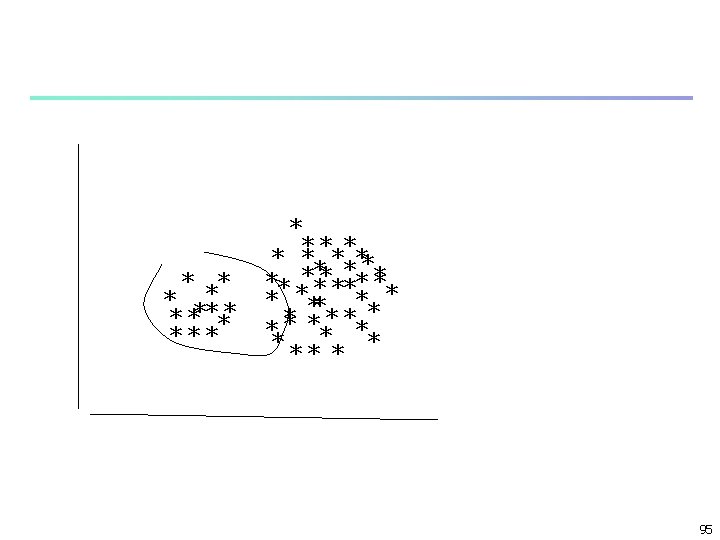
A classification problem in that decision trees are not suitable to classify income A o o o x x o o The two classes X and O are separated by line AA x x o A x x Decision trees are not suitabe For this problem age 42

Exercise n n n Can information gain be negative? Consider a data set wih a binary output such as in the previous example (an attribute with two values: buy not buy) Suppose an input candidatre variable has two values such as Student or credit rating in the previous example. If this variable is selected and branches are formed accodingly A) what is the worst case- the variable is totally unrelated to explain the output? What is the information gain B) What if the variable is most related - highest information gain. 43
 n n On a probability – entropy graph indicate the two")
Exercise (cont. ) n n On a probability – entropy graph indicate the two extreams n Mark on the graph, the entropies of left and right branches, the weighted entropy. Benefiting from the concavity of the entropy function show that information gain can not take a negative value. 44

Chapter 2: Basic Data Mining Techniques n n n Decision Trees: ID 3 Algorithm Association Rule Mining: Apriori Algorithm Clustering: K-Means Algorıthm 45

What Is Association Mining? Association rule mining: n Finding frequent patterns, associations, correlations, or causal structures among sets of items or objects in transaction databases, relational databases, and other information repositories. n Applications: n Market basket analysis, cross-marketing, catalog design, etc. n Examples. n Rule form: “Body Head [support, confidence]”. n buys(x, “diapers”) buys(x, “beers”) [0. 5%, 60%] n major(x, “MIS”) ^ takes(x, “DM”) grade(x, “AA”) [1%, 75%] n 46
 database of transactions, n (2)")
Association Rule: Basic Concepts n n Given: n (1) database of transactions, n (2) each transaction is a list of items (purchased by a customer in a visit) Find: all rules that correlate the presence of one set of items with that of another set of items n E. g. , 98% of people who purchase tires and auto accessories also get automotive services done n The user specifies n Minimum support level n Minimum confidence level n Rules exceeding the two trasholds are listed as interesting 47

Basic Concepts cont. n n n I: {i 1, . . , im} set of all items, T any transaction A T: T contains the itemset A A T, B T A, B itemsets Examine rule like: A B where A B= , n support s: P(A B) n n frequency of transactions containing both A and B confidence c: P(B A) = P(A B)/P(A) n Conditional probability that a transaction containing A contains B 48

Rule Measures: Support and Confidence Customer buys both Customer buys beer Customer n buys diaper Find all the rules X & Y Z with minimum confidence and support n support, s, probability that a transaction contains {X Y Z} n confidence, c, conditional probability that a transaction having {X Y} also contains Z Let minimum support 50%, and minimum confidence 50%, we have n A C (50%, 66. 6%) n C A (50%, 100%) 49

Frequent itemsets n n n n Strong association rules: n Support rule > min_support n Confidence rule > min_confidence k-item set: itemsets containing k items occurrence frequency=count=support count: Minimum support count = min_sup*#transactions in database frequent item sets: n İtemsets satisfying minimum support count The Apriori Algorithm has two steps: n (1) - Find all frequent itemsets n (2) - Genertate strong association rules from frequent itemsets 50
 Min_support 50% Min. _confidence 50% Min_count: 0. 5*4=2 {A}. {B}.")
Mining Association Rules—An Example(1) Min_support 50% Min. _confidence 50% Min_count: 0. 5*4=2 {A}. {B}. {C}. {D} are 1 -itemsets {A}. {B}. {C} are frequent 1 -itemsets as Count[{A}] = 3 >= 2 (minimum_count) or Support[{A}] = 75% >= 50% (minimum_support) {D} is not a frequent 1 -itemsets as Count[{D}] = 1 < 2 (minimum_count) or Support[{D}] = 25% < 50% (minimum_support) 51
 Min_support 50% Min. _confidence 50% Min_count: 0. 5*4=2 {A. B}.")
Mining Association Rules—An Example(2) Min_support 50% Min. _confidence 50% Min_count: 0. 5*4=2 {A. B}. {A. C}. {A. D}. {B. C} are 2 -itemsets {A. C}is frequent 2 -itemsets as Count[{A. C}] = 2 >= 2 (minimum_count) or Support[{A. C}] = 50% >= 50% (minimum_support) {A. B}. {A. D} are not frequent 2 -itemsets as Count[{A. D}] = 1 < 2 (minimum_count) or Support[{A. D}] = 25% < 50% (minimum_support) 52
 Min. support 50% Min. confidence 50% For rule A C:")
Mining Association Rules—An Example(3) Min. support 50% Min. confidence 50% For rule A C: support = support({A C}) = 50% confidence = support({A C})/support({A}) = 66. 6% Strong rule as support >=min_support confidence >= min_confidence 53

The Apriori Principle Min. support 50% Min. confidence 50% The Apriori principle: Any subset of a frequent itemset must be frequent {A. C} is a frequent 2 -itemset {A} and {C}: subsets of {A, C} must be frequent itemsets 1 - 54
-Find the frequent itemsets: the sets of items")
Apriori Algorithme has two steps n (1)-Find the frequent itemsets: the sets of items that have minimum support (the key step) n A subset of a frequent itemset must also be a frequent itemset n n Iteratively find frequent itemsets with cardinality from 1 to k (kitemset) n n i. e. , if {AB} is a frequent itemset, both {A} and {B} should be a frequent itemsets Until k is an empty set (2)-Use the frequent itemsets to generate association rules. 55
 n C 1 L 1")
Generation of frequent itemsets from candidate itemsets (Step 1) n C 1 L 1 C 2 L 2 C 3 L 3 C 4 L 4… n From Ck (candidate k-itemsets) generate Lk : Ck Lk n n From candidate k itemsets generate frequent k itemsets (a)-Using the Apriori principle that: n Eliminate itemset sk in Ck if n n (b)-For candidate k itemsets in Ck n n At least one k-1 subset of sk is not in Lk-1 Make a database scan to eliminate those itemsets whose support counts are below the critical min support cout From frequent k itemsets Lk generate candidate k+1 itemsets Ck+1 : Lk Ck+1 n Self joining any Lk with Lk 56

Self Join operation n n n Sort the items in any li Lk in some lexicographic order n li[1]<li[2]<, … <li[k-1]<li[k] li and lj are elements of Lk li. lj Lk If li[1]=lj[1] and li[2]=lj[2] and … li[k-1]=lj[k-1] and li[k]<lj[k] n The first k-1 elements are the same n Only the last elements are different li lj satisfiing the above condition Construct the item set lk+1: n li[1], li[2], … li[k-1], li[k], lj[k] n common items n the k-1 items are taken form li or lj n k th item is taken from li n k+1 th item is from lj 57

Example of Self Join operation n Lexigographic order: alphabetic a<b<c<d. . n L 3={abc, abd, ace, bcd} n Self-joining: L 3*L 3 Step(2) n n abcd from abc and abd n acde from acd and ace Pruning by Apriori principle: Step(1 a) n n acde is removed because ade is not in L 3 C 4={abcd} 58

The Apriori Algorithm — Example min support cont=2 Database D L 1 C 1 Scan D C 2 Scan D L 2 C 3 Scan D L 3 59

Example 6. 1 Han TID_____list of item_Ids n T 100 125 9 transactions n T 200 24 D=9 n T 300 23 minimum transaction n T 400 124 support_count=2 n T 500 13 min_sup=2/9=22% n T 600 23 n T 700 13 min conf: 70% n T 800 1235 n T 900 123 Find strong association rules: having min sup count of 2 and min confidence %70 n 60

Data Dictionary n n n 1: 2: 3: 4: 5: milk apple butter bread orange 61

1 th iteration of algorithm n n n C 1: itemset sup_count L 1: itemset n 1 6 1 n 2 7 2 n 3 6 3 n 4 2 4 n 5 2 5 sup_count 6 7 6 2 2 C 2: L 1 join L 1, itemset sup_count 1 1 2 2 2 3 3 4 2 3 4 5 4 5 5 4 4 1 x 2 4 2 2 0 x 1 x 0 x L 2 itset supcount 12 4 13 4 15 2 23 4 24 2 25 2 frequent 2 item sets L 2 those itemsets in C 2 having minimum support Step (1 b) 62
")
3 th iteration n n n Self join to get C 3 Step (2) C 3: L 2 join L 2: [1 2 3], [1 2 5], [1 3 5], [2 3 4], [2 3 5], [2 4 5] Now Step (1 a) Apply Apriori to every itemset in C 3 2 item subsets of [1 2 3]: [1 2], [1 3], [2 3] n all 2 items sets are members of L 2 n keep [1 2 3] in C 3 2 item subsets of [1 2 5]: [1 2], [1 5], [2 5] n all 2 items sets are members of L 2 n keep [1 2 5] in C 3 2 item subsets of [1 3 5]: [1 3], [1 5], [3 5] n [3 5] is not a members of L 2 so it si not frequent n remove [1 2 5] from C 3 63
![3 iteration cont. n n 2 item subsets of [2 3 4]: [2 3],](http://slidetodoc.com/presentation_image_h/b9e291b040005587a5a1cd6654438025/image-64.jpg "3 iteration cont. n n 2 item subsets of [2 3 4]: [2 3],")
3 iteration cont. n n 2 item subsets of [2 3 4]: [2 3], [2 4], [3 4] n [3 4] is not a members of L 2 so it si not frequent n remove [2 3 4] from C 3 2 item subsets of [2 3 5]: [2 3], [2 5], [3 5] n [3 5] is not a members of L 2 so it si not frequent n remove [2 3 5] from C 3 2 item subsets of [2 4 5]: [2 4], [2 5], [4 5] n [4 5] is not a members of L 2 so it si not frequent n remove [2 4 5] from C 3: [1 2 3], [1 2 5] after pruning 64

4 th iteration n n n n C 3 L 3 check min support Step (1 b) L 3: those item sets having minimum support L 3: item sets minsupcount n 1 2 3 2 n 1 2 5 2 L 3 join L 3 to generate C 4 Step (2) L 3 join L 3: 1 2 3 5 pruned since its subset [2 3 5] is not frequent C 4= the algorithm terminates 65

Generating Association Rules from frequent itemsets n n Strong rules n min support and min confidence(A B)= P(B A): sup_count(A B) sup_count(A) for each frequent itemset l n generate non empty subsets of l: denoted by s n For each s l n n construct rules: s (l-s) Satısfying the condition: n n sup_count(l)/sup_count(s)>=min_conf are listed as interestıng 66

Example 6. 2 Han cont. n n the 3 -frequent item set l: [1 2 5] non empty subsets of l are n [1 2], [1 5], [2 5], [1], [2], [5] the resulting association rules are: n 1 2 5 conf: 2/4=50% n 1 5 2 conf: 2/2=100% n 2 5 1 conf: 2/2=100% n 1 2 5 conf: 2/6=33% n 2 1 5 conf: 2/7=29% n 5 1 2 conf: 2/2=100% if min conf: 70% 2 th 3 th and last rules are strong 67

Example 6. 2 cont. Detail on confidence for two rules n n n n For the rule 1 5 2 conf: s(1, 2, 5)/s(1, 5) conf: 2/2=100% >= 70% A strong rule For the rule 2 1 5 conf: s(1, 2, 5)/s(2) conf: 2/7=29% < 70% Not a strong rule 68

Exercise n Find all strong association rules in Example 6. 2 n Check minimum confindence n for 2 -frequent intemsets n n [1, 2], [1, 3], [1, 5], [2, 3], [2, 4], [2, 5] 1 2, 2 1 2 5, 5 2 exetra for 3 -frequent intemset n n n [1, 2, 5] 1 2 3 3 1 2 exetra 69
 Suppose A B and B C are strong")
Exercise n n n n a) Suppose A B and B C are strong rules Dose this imply that A C is also a strong rule? b) Suppose A C and B C are strong rules Dose this imply that A AND B C is also a strong rule? c) Suppose A B and A C are strong rules Dose this imply that A B AND C is also a strong? d) Suppose A B AND C is a strong rule. Dose this imply that A B and A C are strong rules? e) Suppose A AND B C is a strong rule. Dose this imply that A C and B C are strong rules? 70
 Suppose {A, B, C} is a frequent 3 itemset.")
Exercise n n n a) Suppose {A, B, C} is a frequent 3 itemset. Dose it imply that {A, B} and {A, C} are frequent 2 itemsets? b) Suppose {A, B}, {A, C}, and {B, C} are frequent 2 itemsets. Dose it imply that {A, B, C} is a frequent 3 itemset? c) Suppose {A, B} is a frequent 2 itemset. Dose it imply that, A B and B A are strong rules? 71

Exercise n n n n Suppose ABCD is a 4 -frequent itemset AB and CD are 2 -frequent itemsets Lexicographic orderıng is based on alphabetıcal order A>B>C>D Since apriri algorithm joıns 2 -frequent itemsets to find 3 candidates But it can not join AB and CD it may miss to identify ABCD as a 4 -frequent itemset Is thıs statement true or false? Or is it possible to miss any k-frequent itemset by the apriori algorithm? 72

Chapter 2: Basic Data Mining Techniques n Decision Trees: ID 3 Algorithm n Association Rule Mining: Apriori Algorithm n Clustering: K-Means Algorıthm 73

What is Cluster Analysis? n n Cluster: a collection of data objects n Similar to one another within the same cluster n Dissimilar to the objects in other clusters Cluster analysis n Finding similarities between data according to the characteristics found in the data and grouping similar data objects into clusters Clustering is unsupervised classification: no predefined classes Typical applications n As a stand-alone tool to get insight into data distribution n As a preprocessing step for other algorithms n Measuring the performance of supervised learning algorithms 74

Basic Measures for Clustering n Clustering: Given a database D = {t 1, t 2, . . , tn}, a distance measure dis(ti, tj) defined between any two objects ti and tj, and an integer value k, the clustering problem is to define a mapping f: D {1, …, k } where each ti is assigned to one cluster Kf, 1 ≤ f ≤ k, 75

Partitioning Algorithms: Basic Concept n n Partitioning method: Construct a partition of a database D of n objects into a set of k clusters, s. t. , min sum of squared distance Given a k, find a partition of k clusters that optimizes the chosen partitioning criterion n Global optimal: exhaustively enumerate all partitions n Heuristic methods: k-means and k-medoids algorithms n k-means (Mac. Queen’ 67): Each cluster is represented by the center of the cluster n k-medoids or PAM (Partition around medoids) (Kaufman & Rousseeuw’ 87): Each cluster is represented by one of the objects in the cluster 76

The K-Means Clustering Algorithm n choose k, number of clusters to be determined n Choose k objects randomly as the initial cluster centers n repeat n Assign each object to their closest cluster center n n Compute new cluster centers n n Using Euclidean distance Calculate mean points until n No change in cluster centers or n No object change its cluster 77

The K-Means Clustering Method n Example 10 10 9 9 8 8 7 7 6 6 5 5 4 3 2 1 0 0 1 2 3 4 5 6 7 8 9 10 Assign each objects to most similar center Update the cluster means reassign 4 3 2 1 0 0 1 2 3 4 5 6 7 8 9 10 reassign K=2 Arbitrarily choose K object as initial cluster center Update the cluster means 78

Example TBP Sec 3. 3 page 84 Table 3. 6 n n n Instance X Y n 1 1. 0 1. 5 n 2 1. 0 4. 5 n 3 2. 0 1. 5 n 4 2. 0 3. 5 n 5 3. 0 2. 5 n 6 5. 0 6. 1 k is chosen as 2 k=2 Chose two points at random representing initial cluster centers n Object 1 and 3 are chosen as cluster centers 79

Example cont. n n n Euclidean distance between point i and j D(i - j)=( (Xi – Xj)2 + (Yi – Yj)2)1/2 Initial cluster centers n C 1: (1. 0, 1. 5) C 2: (2. 0, 1. 5) D(C 1 – 1) = 0. 00 n D(C 1 – 2) = 3. 00 n D(C 1 – 3) = 1. 00 n D(C 1 – 4) = 2. 24 n D(C 1 – 5) = 2. 24 n D(C 1 – 6) = 6. 02 C 1: {1, 2} C 2: {3. 4. 5. 6} n n D(C 2 D(C 2 – 1) – 2) – 3) – 4) – 5) – 6) = = = 1. 00 3. 16 0. 00 2. 00 1. 41 5. 41 C 1 C 2 C 2 80

6 2 4 5 1* 3* 81

Example cont. n n n Recomputing cluster centers For C 1: n XC 1 = (1. 0+1. 0)/2 = 1. 0 n YC 1 = (1. 5+4. 5)/2 = 3. 0 For C 2: n XC 2 = (2. 0+3. 0+5. 0)/4 = 3. 0 n YC 2 = (1. 5+3. 5+2. 5+6. 0)/4 = 3. 375 Thus the new cluster centers are C 1(1. 0, 3. 0) and C 2(3. 0, 3. 375) As the cluster centers have changed n The algorithm performs another iteration 82

6 2 4 5 1* 3* 83
 and C 2(3.")
Example cont. n New cluster centers C 1(1. 0, 3. 0) and C 2(3. 0, 3. 375) n D(C 1 – 1) = 1. 50 n D(C 1 – 2) = 1. 50 n D(C 1 – 3) = 1. 80 n D(C 1 – 4) = 1. 12 n D(C 1 – 5) = 2. 06 n D(C 1 – 6) = 5. 00 C 1 {1, 2. 3} C 2: {4. 5. 6} n n D(C 2 D(C 2 – 1) – 2) – 3) – 4) – 5) – 6) = = = 2. 74 2. 29 2. 13 1. 01 0. 88 3. 30 C 1 C 1 C 2 C 2 84

6 2 * * 4 5 1 3 85

Example cont. n n n computing new cluster centers For C 1: n XC 1 = (1. 0+2. 0)/3 = 1. 33 n YC 1 = (1. 5+4. 5+1. 5)/3 = 2. 50 For C 2: n XC 2 = (2. 0+3. 0+5. 0)/3 = 3. 33 n YC 2 = (3. 5+2. 5+6. 0)/3 = 4. 00 Thus the new cluster centers are C 1(1. 33, 2. 50) and C 2(3. 33, 4. 3. 00) As the cluster centers have changed n The algorithm performs another iteration 86

Exercise n Perform the third iteration 87

Commands n n n each initial cluster centers may end up with different final cluster configuration Finds local optimum but not necessarily the global optimum n Based on sum of squared error SSE differences between objects and their cluster centers Choose a terminating criterion such as n Maximum acceptable SSE n Execute K-Means algorithm until satisfying the condition 88
, where n is #")
Comments on the K-Means Method n Strength: Relatively efficient: O(tkn), where n is # objects, k is # clusters, and t is # iterations. Normally, k, t << n. n n Comparing: PAM: O(k(n-k)2 ), CLARA: O(ks 2 + k(n-k)) Comment: Often terminates at a local optimum. The global optimum may be found using techniques such as: deterministic annealing and genetic algorithms 89

Weaknesses of K-Means Algorithm n n Applicable only when mean is defined, then what about categorical data? Need to specify k, the number of clusters, in advance n run the algorithm with different k values n Unable to handle noisy data and outliers n Not suitable to discover clusters with non-convex shapes n Works best when clusters are of approximately of equal size 90

Presence of Outliers x x xx xx x When k=2 x x xx xx x When k=3 When k=2 the two natural clusters are not captured 91

Quality of clustering depends on unit of measure income x x x age Income measured by YTL, age by year x age Income measured by So what to do? TL, age by year 92

Variations of the K-Means Method n n A few variants of the k-means which differ in n Selection of the initial k means n Dissimilarity calculations n Strategies to calculate cluster means Handling categorical data: k-modes (Huang’ 98) n Replacing means of clusters with modes n Using new dissimilarity measures to deal with categorical objects n Using a frequency-based method to update modes of clusters n A mixture of categorical and numerical data: k-prototype method 93
 K-means algorithm may converge to")
Exercise n Show by designing simple examples: n a) K-means algorithm may converge to different local optima starting from different initial assignments of objects into different clusters n b) In the case of clusters of unequal size, Kmeans algorithm may fail to catch the obvious (natural) solution 94
- Slides: 95