MIS 214 Statistics II 20132014 Spring Chapter 6

MIS 214 Statistics II 2013/2014 Spring Chapter 6 7 9 Copyright © 2013 Pearson Education, Inc. Publishing as Prentice Hall Ch. 6 -1

Chapter Goals After completing this chapter, you should be able to: n Describe a simple random sample and why sampling is important n Explain the difference between descriptive and inferential statistics n Define the concept of a sampling distribution n Determine the mean and standard deviation for the sampling distribution of the sample mean, n Describe the Central Limit Theorem and its importance n Determine the mean and standard deviation for the sampling distribution of the sample proportion, n Describe sampling distributions of sample variances Copyright © 2013 Pearson Education, Inc. Publishing as Prentice Hall Ch. 6 -2

Introduction n Descriptive statistics n n Collecting, presenting, and describing data Inferential statistics n Drawing conclusions and/or making decisions concerning a population based only on sample data Copyright © 2013 Pearson Education, Inc. Publishing as Prentice Hall Ch. 6 -3

Inferential Statistics n Making statements about a population by examining sample results Sample statistics (known) Population parameters Inference Copyright © 2013 Pearson Education, Inc. Publishing as Prentice Hall (unknown, but can be estimated from sample evidence) Ch. 6 -4

Inferential Statistics Drawing conclusions and/or making decisions concerning a population based on sample results. n Estimation n n e. g. , Estimate the population mean weight using the sample mean weight Hypothesis Testing n e. g. , Use sample evidence to test the claim that the population mean weight is 120 pounds Copyright © 2013 Pearson Education, Inc. Publishing as Prentice Hall Ch. 6 -5

6. 1 n Sampling from a Population A Population is the set of all items or individuals of interest n n Examples: All likely voters in the next election All parts produced today All sales receipts for November A Sample is a subset of the population n Examples: 1000 voters selected at random for interview A few parts selected for destructive testing Random receipts selected for audit Copyright © 2013 Pearson Education, Inc. Publishing as Prentice Hall Ch. 6 -6

Population vs. Sample Population Copyright © 2013 Pearson Education, Inc. Publishing as Prentice Hall Sample Ch. 6 -7

Why Sample? n Less time consuming than a census n Less costly to administer than a census n It is possible to obtain statistical results of a sufficiently high precision based on samples. Copyright © 2013 Pearson Education, Inc. Publishing as Prentice Hall Ch. 6 -8

Simple Random Sample n n Every object in the population has the same probability of being selected Objects are selected independently Samples can be obtained from a table of random numbers or computer random number generators A simple random sample is the ideal against which other sampling methods are compared Copyright © 2013 Pearson Education, Inc. Publishing as Prentice Hall Ch. 6 -9

Sampling Distributions n A sampling distribution is a probability distribution of all of the possible values of a statistic for a given size sample selected from a population Copyright © 2013 Pearson Education, Inc. Publishing as Prentice Hall Ch. 6 -10

Chapter Outline Sampling Distributions of Sample Means Sampling Distributions of Sample Proportions Copyright © 2013 Pearson Education, Inc. Publishing as Prentice Hall Sampling Distributions of Sample Variances Ch. 6 -11

6. 2 Sampling Distributions of Sample Means Sampling Distributions of Sample Proportions Copyright © 2013 Pearson Education, Inc. Publishing as Prentice Hall Sampling Distributions of Sample Variances Ch. 6 -12

Sample Mean n n Let X 1, X 2, . . . , Xn represent a random sample from a population The sample mean value of these observations is defined as Copyright © 2013 Pearson Education, Inc. Publishing as Prentice Hall Ch. 6 -13

Standard Error of the Mean n Different samples of the same size from the same population will yield different sample means A measure of the variability in the mean from sample to sample is given by the Standard Error of the Mean: Note that the standard error of the mean decreases as the sample size increases Copyright © 2013 Pearson Education, Inc. Publishing as Prentice Hall Ch. 6 -14

If sample values are not independent n n n If the sample size n is not a small fraction of the population size N, then individual sample members are not distributed independently of one another Thus, observations are not selected independently A finite population correction is made to account for this: or The term (N – n)/(N – 1) is often called a finite population correction factor Copyright © 2013 Pearson Education, Inc. Publishing as Prentice Hall Ch. 6 -15

n n n If the sample size n is a small fraction of the population size N, then individual sample members are distributed independently of one another Let X 1, X 2, … Xn is a random sample from a poplation, Each Xi is a random variable whose parameters are the same as populations n n Fixed and unknown In parametric frequencist paradigm of inference n n Assume a distrinutional form for population Take a random sample from the population

If the Population is Normal n If a population is normal with mean μ and standard deviation σ, the sampling distribution of is also normally distributed with and n If the sample size n is not large relative to the population size N, then and Copyright © 2013 Pearson Education, Inc. Publishing as Prentice Hall Ch. 6 -17

Standard Normal Distribution for the Sample Means n Z-value for the sampling distribution of where: : = sample mean = population mean = standard error of the mean Z is a standardized normal random variable with mean of 0 and a variance of 1 Copyright © 2013 Pearson Education, Inc. Publishing as Prentice Hall Ch. 6 -18

Sampling Distribution Properties Normal Population Distribution (i. e. is unbiased ) Normal Sampling Distribution (both distributions have the same mean) Copyright © 2013 Pearson Education, Inc. Publishing as Prentice Hall Ch. 6 -19

Sampling Distribution Properties (continued) Normal Population Distribution (i. e. is unbiased ) (the distribution of standard deviation Normal Sampling Distribution has a reduced Copyright © 2013 Pearson Education, Inc. Publishing as Prentice Hall Ch. 6 -20

Sampling Distribution Properties (continued) As n increases, decreases Larger sample size Smaller sample size Copyright © 2013 Pearson Education, Inc. Publishing as Prentice Hall Ch. 6 -21

Central Limit Theorem n n Even if the population is not normal, …sample means from the population will be approximately normal as long as the sample size is large enough. Copyright © 2013 Pearson Education, Inc. Publishing as Prentice Hall Ch. 6 -22

Central Limit Theorem (continued) n n Let X 1, X 2, . . . , Xn be a set of n independent random variables having identical distributions with mean µ, variance σ2, and X as the mean of these random variables. As n becomes large, the central limit theorem states that the distribution of approaches the standard normal distribution Copyright © 2013 Pearson Education, Inc. Publishing as Prentice Hall Ch. 6 -23

Central Limit Theorem As the sample size gets large enough… n↑ Copyright © 2013 Pearson Education, Inc. Publishing as Prentice Hall the sampling distribution becomes almost normal regardless of shape of population Ch. 6 -24

If the Population is not Normal (continued) Sampling distribution properties: Population Distribution Central Tendency Variation Sampling Distribution (becomes normal as n increases) Smaller sample size Copyright © 2013 Pearson Education, Inc. Publishing as Prentice Hall Larger sample size Ch. 6 -25

How Large is Large Enough? n n For most distributions, n > 25 will give a sampling distribution that is nearly normal For normal population distributions, the sampling distribution of the mean is always normally distributed Copyright © 2013 Pearson Education, Inc. Publishing as Prentice Hall Ch. 6 -26

Example n n Suppose a large population has mean μ = 8 and standard deviation σ = 3. Suppose a random sample of size n = 36 is selected. What is the probability that the sample mean is between 7. 8 and 8. 2? Copyright © 2013 Pearson Education, Inc. Publishing as Prentice Hall Ch. 6 -27

Example (continued) Solution: n n Even if the population is not normally distributed, the central limit theorem can be used (n > 25) … so the sampling distribution of approximately normal n … with mean n …and standard deviation is = 8 Copyright © 2013 Pearson Education, Inc. Publishing as Prentice Hall Ch. 6 -28

Example (continued) Solution (continued): Population Distribution ? ? ? Sampling Distribution Standard Normal Distribution Sample ? X . 1554 +. 1554 Standardize 7. 8 Copyright © 2013 Pearson Education, Inc. Publishing as Prentice Hall 8. 2 -0. 4 Z Ch. 6 -29

Acceptance Intervals n Goal: determine a range within which sample means are likely to occur, given a population mean and variance n n n By the Central Limit Theorem, we know that the distribution of X is approximately normal if n is large enough, with mean μ and standard deviation Let zα/2 be the z-value that leaves area α/2 in the upper tail of the normal distribution (i. e. , the interval - zα/2 to zα/2 encloses probability 1 – α) Then is the interval that includes X with probability 1 – α Copyright © 2013 Pearson Education, Inc. Publishing as Prentice Hall Ch. 6 -30

6. 3 Sampling Distributions of Sample Proportions Sampling Distributions of Sample Means Sampling Distributions of Sample Proportions Copyright © 2013 Pearson Education, Inc. Publishing as Prentice Hall Sampling Distributions of Sample Variances Ch. 6 -31

Sampling Distributions of Sample Proportions P = the proportion of the population having some characteristic n n n Sample proportion ( ) provides an estimate of P: 0≤ ≤ 1 has a binomial distribution, but can be approximated by a normal distribution when n. P(1 – P) > 5 Copyright © 2013 Pearson Education, Inc. Publishing as Prentice Hall Ch. 6 -32

^ Sampling Distribution of p n Normal approximation: Sampling Distribution. 3. 2. 1 0 0 . 2 . 4 . 6 8 1 Properties: and (where P = population proportion) Copyright © 2013 Pearson Education, Inc. Publishing as Prentice Hall Ch. 6 -33

Z-Value for Proportions Standardize to a Z value with the formula: Where the distribution of Z is a good approximation to the standard normal distribution if n. P(1−P) > 5 Copyright © 2013 Pearson Education, Inc. Publishing as Prentice Hall Ch. 6 -34

Example n If the true proportion of voters who support Proposition A is P = 0. 4, what is the probability that a sample of size 200 yields a sample proportion between 0. 40 and 0. 45? § i. e. : if P = 0. 4 and n = 200, what is P(0. 40 ≤ Copyright © 2013 Pearson Education, Inc. Publishing as Prentice Hall ≤ 0. 45) ? Ch. 6 -35

Example (continued) if P = 0. 4 and n = 200, what is P(0. 40 ≤ ≤ 0. 45) ? n Find : Convert to standard normal: Copyright © 2013 Pearson Education, Inc. Publishing as Prentice Hall Ch. 6 -36

Example (continued) n if P = 0. 4 and n = 200, what is P(0. 40 ≤ ≤ 0. 45) ? Use standard normal table: P(0 ≤ Z ≤ 1. 44) =. 4251 Standardized Normal Distribution Sampling Distribution . 4251 Standardize . 40 . 45 Copyright © 2013 Pearson Education, Inc. Publishing as Prentice Hall 0 1. 44 Z Ch. 6 -37

Statistics for Business and Economics 8 th Edition Chapter 7 Estimation: Single Population Copyright © 2013 Pearson Education, Inc. Publishing as Prentice Hall Ch. 7 -38

Chapter Goals After completing this chapter, you should be able to: n n n Distinguish between a point estimate and a confidence interval estimate Construct and interpret a confidence interval estimate for a single population mean using both the Z and t distributions Form and interpret a confidence interval estimate for a single population proportion Create confidence interval estimates for the variance of a normal population Determine the required sample size to estimate a mean or proportion within a specified margin of error Copyright © 2013 Pearson Education, Inc. Publishing as Prentice Hall Ch. 7 -39

Confidence Intervals Contents of this chapter: n Confidence Intervals for the Population Mean, μ n n n when Population Variance σ2 is Known when Population Variance σ2 is Unknown Confidence Intervals for the Population Proportion, P (large samples) Confidence interval estimates for the variance of a normal population Finite population corrections Sample-size determination Copyright © 2013 Pearson Education, Inc. Publishing as Prentice Hall Ch. 7 -40

7. 1 n Properties of Point Estimators An estimator of a population parameter is n n n a random variable that depends on sample information. . . whose value provides an approximation to this unknown parameter A specific value of that random variable is called an estimate Copyright © 2013 Pearson Education, Inc. Publishing as Prentice Hall Ch. 7 -41

Point and Interval Estimates n n A point estimate is a single number, a confidence interval provides additional information about variability Lower Confidence Limit Point Estimate Upper Confidence Limit Width of confidence interval Copyright © 2013 Pearson Education, Inc. Publishing as Prentice Hall Ch. 7 -42

Point Estimates We can estimate a Population Parameter … Mean μ Proportion P Copyright © 2013 Pearson Education, Inc. Publishing as Prentice Hall with a Sample Statistic (a Point Estimate) x Ch. 7 -43

Unbiasedness n n A point estimator is said to be an unbiased estimator of the parameter if its expected value is equal to that parameter: Examples: n The sample mean is an unbiased estimator of μ 2 2 n The sample variance s is an unbiased estimator of σ n The sample proportion is an unbiased estimator of P Copyright © 2013 Pearson Education, Inc. Publishing as Prentice Hall Ch. 7 -44

Unbiasedness (continued) n is an unbiased estimator, Copyright © 2013 Pearson Education, Inc. Publishing as Prentice Hall is biased: Ch. 7 -45

Bias n n n Let be an estimator of The bias in is defined as the difference between its mean and The bias of an unbiased estimator is 0 Copyright © 2013 Pearson Education, Inc. Publishing as Prentice Hall Ch. 7 -46

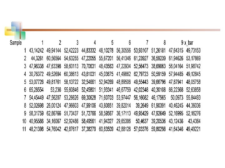
Exercise n n n n In the previous exampleof student grades Population: mean 50, variance 100 or std 10 We took samples of size 9 Compute sample means x_bar Replicated this 1000 times Average of these sample meands is almost 50 Standard dev. Of these x_bars is about 10/3

n n n n From N(50, 10) n=9 Each raw is a sample of size 9 Then x_bar is computed in last colomn Draw histogram for x_bar s It is N(50, 3. 33) In reality only one sample is taken – Hypothetical – go back in time repeat the exam Due to randomness -

n n n Assume grades are from a population Assume a distributional form Parameters are unknown Aim of infrential statistics is Estimation of the fixed but unknown parameters Ther is no way to know the values of the population parameters

A simple high school problem n n Ahmets age is 2 times Ayses age Sum of their ages is 30 What are Ahmet and Ayşe s ages? Ages are fixed unknown, n n At the begining When the prblem is solved n Determine the values

but n n n In th frquencist parametric paradigm Population parameters are fixed bt unknown as well But ther is no way to find their values At best what can be done Estimate those paramters n n Point or intervfal estimates Test your clames on these parameters

Population distributons n n n n n Hypothesize distributional forms Test these hypothesis Godness of fit tests chapter 14 If normality of populations is rejected For large ssmle sizes İnference about mean is based on x: bar Central limit theorem Infrence about variance or tests based on variance Use nonparametric tests

Exercise n n n Population normal mean 50, std 10 samle size – n: 3 Replicate 1000 times n n n Generate 3 N(50, 10) grades Compute x_bar Compute 3 i=1(xi-x_bar)2 Compute average of these 3 i=1(xi-x_bar)2 Almost 200 = (n-1)*102 n n n E[ 3 i=1(xi-x_bar)2] = (n-1) 2 Or E[ 3 i=1(xi-x_bar)2/ (n-1)] = 2

Exercise n n n Population normal mean 50, std 10 sample size – n: 3 Replicate 1000 times n n n Generate 3 N(50, 10) grades Compute x_bar Compute 3 i=1(xi- )2 Compute average of these 3 i=1(xi-x_bar)2 Almost 300 = (n-1)*102 n n n E[ 3 i=1(xi- )2] = (n) 2 Or E[ 3 i=1(xi-x_bar)2/ (n)] = 2

n n If the population of grades is uniform rather then normal The statistic 3 i=1(xi-x_bar)2/ 2 is not chi-square at all

Confidence Interval Estimation n How much uncertainty is associated with a point estimate of a population parameter? An interval estimate provides more information about a population characteristic than does a point estimate Such interval estimates are called confidence interval estimates Copyright © 2013 Pearson Education, Inc. Publishing as Prentice Hall Ch. 7 -57

Confidence Interval Estimate n An interval gives a range of values: n n Takes into consideration variation in sample statistics from sample to sample Based on observation from 1 sample Gives information about closeness to unknown population parameters Stated in terms of level of confidence n Can never be 100% confident Copyright © 2013 Pearson Education, Inc. Publishing as Prentice Hall Ch. 7 -58

Confidence Interval and Confidence Level n n If P(a < < b) = 1 - then the interval from a to b is called a 100(1 - )% confidence interval of . The quantity 100(1 - )% is called the confidence level of the interval n n n is between 0 and 1 In repeated samples of the population, the true value of the parameter would be contained in 100(1 - )% of intervals calculated this way. The confidence interval calculated in this manner is written as a < < b with 100(1 - )% confidence Copyright © 2013 Pearson Education, Inc. Publishing as Prentice Hall Ch. 7 -59

Estimation Process Random Sample Population (mean, μ, is unknown) Mean X = 50 I am 95% confident that μ is between 40 & 60. Sample Copyright © 2013 Pearson Education, Inc. Publishing as Prentice Hall Ch. 7 -60

Confidence Level, (1 - ) (continued) n n n Suppose confidence level = 95% Also written (1 - ) = 0. 95 A relative frequency interpretation: n n From repeated samples, 95% of all the confidence intervals that can be constructed of size n will contain the unknown true parameter A specific interval either will contain or will not contain the true parameter n No probability involved in a specific interval Copyright © 2013 Pearson Education, Inc. Publishing as Prentice Hall Ch. 7 -61

General Formula n The general form for all confidence intervals is: Point Estimate Margin of Error n The value of the margin of error depends on the desired level of confidence Copyright © 2013 Pearson Education, Inc. Publishing as Prentice Hall Ch. 7 -62

Confidence Intervals Population Mean σ2 Known Population Proportion Population Variance σ2 Unknown (From normally distributed populations) Copyright © 2013 Pearson Education, Inc. Publishing as Prentice Hall Ch. 7 -63

Confidence Interval Estimation for the Mean (σ2 Known) 7. 2 n Assumptions n n Population variance σ2 is known Population is normally distributed If population is not normal, use large sample Confidence interval estimate: (where z /2 is the normal distribution value for a probability of /2 in each tail) Copyright © 2013 Pearson Education, Inc. Publishing as Prentice Hall Ch. 7 -64

Confidence Limits n The confidence interval is n The endpoints of the interval are Upper confidence limit Lower confidence limit Copyright © 2013 Pearson Education, Inc. Publishing as Prentice Hall Ch. 7 -65

Margin of Error n n n The confidence interval, Can also be written as where ME is called the margin of error The interval width, w, is equal to twice the margin of error Copyright © 2013 Pearson Education, Inc. Publishing as Prentice Hall Ch. 7 -66

Reducing the Margin of Error The margin of error can be reduced if n the population standard deviation can be reduced (σ↓) n The sample size is increased (n↑) n The confidence level is decreased, (1 – ) ↓ Copyright © 2013 Pearson Education, Inc. Publishing as Prentice Hall Ch. 7 -67

Finding z /2 n Consider a 95% confidence interval: Z units: X units: z = -1. 96 Lower Confidence Limit 0 Point Estimate z = 1. 96 Upper Confidence Limit § Find z. 025 = 1. 96 from the standard normal distribution table Copyright © 2013 Pearson Education, Inc. Publishing as Prentice Hall Ch. 7 -68

Statistics for Business and Economics 8 th Edition Chapter 9 Hypothesis Testing: Single Population Copyright © 2013 Pearson Education, Inc. Publishing as Prentice Hall Ch. 9 -69

9. 1 n Concepts of Hypothesis Testing A hypothesis is a claim (assumption) about a population parameter: n population mean Example: The mean monthly cell phone bill of this city is μ = $52 n population proportion Example: The proportion of adults in this city with cell phones is P =. 88 Copyright © 2013 Pearson Education, Inc. Publishing as Prentice Hall Ch. 9 -70

The Null Hypothesis, H 0 n States the assumption (numerical) to be tested Example: The average number of TV sets in U. S. Homes is equal to three ( ) n Is always about a population parameter, not about a sample statistic Copyright © 2013 Pearson Education, Inc. Publishing as Prentice Hall Ch. 9 -71

The Null Hypothesis, H 0 (continued) n n Begin with the assumption that the null hypothesis is true n Similar to the notion of innocent until proven guilty Refers to the status quo Always contains “=” , “≤” or “ ” sign May or may not be rejected Copyright © 2013 Pearson Education, Inc. Publishing as Prentice Hall Ch. 9 -72

The Alternative Hypothesis, H 1 n Is the opposite of the null hypothesis n n n e. g. , The average number of TV sets in U. S. homes is not equal to 3 ( H 1: μ ≠ 3 ) Challenges the status quo Never contains the “=” , “≤” or “ ” sign May or may not be supported Is generally the hypothesis that the researcher is trying to support Copyright © 2013 Pearson Education, Inc. Publishing as Prentice Hall Ch. 9 -73

Hypothesis Testing Process Claim: the population mean age is 50. (Null Hypothesis: H 0: μ = 50 ) Population Is x = 20 likely if μ = 50? If not likely, REJECT Null Hypothesis Copyright © 2013 Pearson Education, Inc. Publishing as Prentice Hall Suppose the sample mean age is 20: x = 20 Now select a random sample Sample Ch. 9 -74

Reason for Rejecting H 0 Sampling Distribution of X 20 If it is unlikely that we would get a sample mean of this value. . . μ = 50 If H 0 is true . . . if in fact this were the population mean… Copyright © 2013 Pearson Education, Inc. Publishing as Prentice Hall X . . . then we reject the null hypothesis that μ = 50. Ch. 9 -75

Level of Significance, n Defines the unlikely values of the sample statistic if the null hypothesis is true n n Defines rejection region of the sampling distribution Is designated by , (level of significance) n Typical values are 0. 01, 0. 05, or 0. 10 n Is selected by the researcher at the beginning n Provides the critical value(s) of the test Copyright © 2013 Pearson Education, Inc. Publishing as Prentice Hall Ch. 9 -76

Level of Significance and the Rejection Region Level of significance = H 0: μ = 3 H 1: μ ≠ 3 /2 Two-tail test /2 Represents critical value Rejection region is shaded 0 H 0: μ ≤ 3 H 1: μ > 3 Upper-tail test H 0: μ ≥ 3 H 1: μ < 3 0 Lower-tail test Copyright © 2013 Pearson Education, Inc. Publishing as Prentice Hall 0 Ch. 9 -77

Errors in Making Decisions n Type I Error n Reject a true null hypothesis n Considered a serious type of error The probability of Type I Error is n Called level of significance of the test n Set by researcher in advance Copyright © 2013 Pearson Education, Inc. Publishing as Prentice Hall Ch. 9 -78

Errors in Making Decisions (continued) n Type II Error n Fail to reject a false null hypothesis The probability of Type II Error is β Copyright © 2013 Pearson Education, Inc. Publishing as Prentice Hall Ch. 9 -79

Outcomes and Probabilities Possible Hypothesis Test Outcomes Actual Situation Decision Key: Outcome (Probability) Fail to Reject H 0 True Correct Decision (1 - ) Reject H 0 Type I Error ( ) H 0 False Type II Error (β) Correct Decision (1 -β) ( 1 - β ) is called the power of the test Copyright © 2013 Pearson Education, Inc. Publishing as Prentice Hall Ch. 9 -80

Consequences of Fixing the Significance Level of a Test n Once the significance level α is chosen (generally less than 0. 10), the probability of Type II error, β, can be found. Investigator chooses significance level (probability of Type I error) Decision rule is established Copyright © 2013 Pearson Education, Inc. Publishing as Prentice Hall Probability of Type II error follows Ch. 9 -81

Type I & II Error Relationship § Type I and Type II errors can not happen at the same time § Type I error can only occur if H 0 is true § Type II error can only occur if H 0 is false If Type I error probability ( ) , then Type II error probability ( β ) Copyright © 2013 Pearson Education, Inc. Publishing as Prentice Hall Ch. 9 -82

Factors Affecting Type II Error n All else equal, n β when the difference between hypothesized parameter and its true value n β when σ n β when n Copyright © 2013 Pearson Education, Inc. Publishing as Prentice Hall Ch. 9 -83

Power of the Test n n The power of a test is the probability of rejecting a null hypothesis that is false i. e. , n Power = P(Reject H 0 | H 1 is true) Power of the test increases as the sample size increases Copyright © 2013 Pearson Education, Inc. Publishing as Prentice Hall Ch. 9 -84

Hypothesis Tests for the Mean Hypothesis Tests for Known Copyright © 2013 Pearson Education, Inc. Publishing as Prentice Hall Unknown Ch. 9 -85

9. 2 n Tests of the Mean of a Normal Distribution (σ Known) Convert sample result ( ) to a z value Hypothesis Tests for σ Known σ Unknown Consider the test The decision rule is: (Assume the population is normal) Copyright © 2013 Pearson Education, Inc. Publishing as Prentice Hall Ch. 9 -86

Decision Rule H 0: μ = μ 0 H 1: μ > μ 0 Alternate rule: Z Do not reject H 0 0 zα Reject H 0 μ 0 Copyright © 2013 Pearson Education, Inc. Publishing as Prentice Hall Critical value Ch. 9 -87

p-Value n p-value: Probability of obtaining a test statistic more extreme ( ≤ or ) than the observed sample value given H 0 is true n n Also called observed level of significance Smallest value of for which H 0 can be rejected Copyright © 2013 Pearson Education, Inc. Publishing as Prentice Hall Ch. 9 -88

p-Value Approach to Testing n n n Convert sample result (e. g. , statistic ) ) to test statistic (e. g. , z Obtain the p-value n For an upper tail test: Decision rule: compare the p-value to n If p-value < , reject H 0 n If p-value , do not reject H 0 Copyright © 2013 Pearson Education, Inc. Publishing as Prentice Hall Ch. 9 -89

Example: Upper-Tail Z Test for Mean ( Known) A phone industry manager thinks that customer monthly cell phone bill have increased, and now average over $52 per month. The company wishes to test this claim. (Assume = 10 is known) Form hypothesis test: H 0: μ ≤ 52 the average is not over $52 per month H 1: μ > 52 the average is greater than $52 per month (i. e. , sufficient evidence exists to support the manager’s claim) Copyright © 2013 Pearson Education, Inc. Publishing as Prentice Hall Ch. 9 -90

Example: Find Rejection Region (continued) n Suppose that =. 10 is chosen for this test Find the rejection region: Reject H 0 =. 10 Do not reject H 0 0 Copyright © 2013 Pearson Education, Inc. Publishing as Prentice Hall 1. 28 Reject H 0 Ch. 9 -91

Example: Sample Results (continued) Obtain sample and compute the test statistic Suppose a sample is taken with the following results: n = 64, x = 53. 1 ( = 10 was assumed known) n Using the sample results, Copyright © 2013 Pearson Education, Inc. Publishing as Prentice Hall Ch. 9 -92

Example: Decision (continued) Reach a decision and interpret the result: Reject H 0 =. 10 Do not reject H 0 1. 28 0 z = 0. 88 Reject H 0 Do not reject H 0 since z = 0. 88 < 1. 28 i. e. : there is not sufficient evidence that the mean bill is over $52 Copyright © 2013 Pearson Education, Inc. Publishing as Prentice Hall Ch. 9 -93

Example: p-Value Solution Calculate the p-value and compare to (continued) (assuming that μ = 52. 0) p-value =. 1894 Reject H 0 =. 10 0 Do not reject H 0 1. 28 Z =. 88 Reject H 0 Do not reject H 0 since p-value =. 1894 > =. 10 Copyright © 2013 Pearson Education, Inc. Publishing as Prentice Hall Ch. 9 -94

One-Tail Tests n In many cases, the alternative hypothesis focuses on one particular direction H 0: μ ≤ 3 H 1: μ > 3 H 0: μ ≥ 3 H 1: μ < 3 This is an upper-tail test since the alternative hypothesis is focused on the upper tail above the mean of 3 This is a lower-tail test since the alternative hypothesis is focused on the lower tail below the mean of 3 Copyright © 2013 Pearson Education, Inc. Publishing as Prentice Hall Ch. 9 -95

Upper-Tail Tests n There is only one critical value, since the rejection area is in only one tail H 0: μ ≤ 3 H 1: μ > 3 Do not reject H 0 Z 0 zα Reject H 0 μ Critical value Copyright © 2013 Pearson Education, Inc. Publishing as Prentice Hall Ch. 9 -96

Lower-Tail Tests n There is only one critical value, since the rejection area is in only one tail H 0: μ ≥ 3 H 1: μ < 3 Reject H 0 -z Do not reject H 0 0 Z μ Critical value Copyright © 2013 Pearson Education, Inc. Publishing as Prentice Hall Ch. 9 -97

Two-Tail Tests n n In some settings, the alternative hypothesis does not specify a unique direction There are two critical values, defining the two regions of rejection H 0: μ = 3 H 1: μ ¹ 3 /2 x 3 Reject H 0 Do not reject H 0 -z /2 Lower critical value Copyright © 2013 Pearson Education, Inc. Publishing as Prentice Hall 0 Reject H 0 +z /2 z Upper critical value Ch. 9 -98

Hypothesis Testing Example Test the claim that the true mean # of TV sets in US homes is equal to 3. (Assume σ = 0. 8) n n n State the appropriate null and alternative hypotheses n H 0: μ = 3 , H 1: μ ≠ 3 (This is a two tailed test) Specify the desired level of significance n Suppose that =. 05 is chosen for this test Choose a sample size n Suppose a sample of size n = 100 is selected Copyright © 2013 Pearson Education, Inc. Publishing as Prentice Hall Ch. 9 -99

Hypothesis Testing Example (continued) n n n Determine the appropriate technique n σ is known so this is a z test Set up the critical values n For =. 05 the critical z values are ± 1. 96 Collect the data and compute the test statistic n Suppose the sample results are n = 100, x = 2. 84 (σ = 0. 8 is assumed known) So the test statistic is: Copyright © 2013 Pearson Education, Inc. Publishing as Prentice Hall Ch. 9 -100

Hypothesis Testing Example (continued) n Is the test statistic in the rejection region? Reject H 0 if z < -1. 96 or z > 1. 96; otherwise do not reject H 0 =. 05/2 Reject H 0 -z = -1. 96 =. 05/2 Do not reject H 0 0 Reject H 0 +z = +1. 96 Here, z = -2. 0 < -1. 96, so the test statistic is in the rejection region Copyright © 2013 Pearson Education, Inc. Publishing as Prentice Hall Ch. 9 -101

Hypothesis Testing Example (continued) n Reach a decision and interpret the result =. 05/2 Reject H 0 -z = -1. 96 =. 05/2 Do not reject H 0 0 Reject H 0 +z = +1. 96 -2. 0 Since z = -2. 0 < -1. 96, we reject the null hypothesis and conclude that there is sufficient evidence that the mean number of TVs in US homes is not equal to 3 Copyright © 2013 Pearson Education, Inc. Publishing as Prentice Hall Ch. 9 -102

Example: p-Value n Example: How likely is it to see a sample mean of 2. 84 (or something further from the mean, in either direction) if the true mean is = 3. 0? x = 2. 84 is translated to a z score of z = -2. 0 /2 =. 025 . 0228 p-value =. 0228 +. 0228 =. 0456 Copyright © 2013 Pearson Education, Inc. Publishing as Prentice Hall -1. 96 -2. 0 0 1. 96 2. 0 Z Ch. 9 -103

Example: p-Value n (continued) Compare the p-value with n If p-value < , reject H 0 n If p-value , do not reject H 0 Here: p-value =. 0456 =. 05 Since. 0456 <. 05, we reject the null hypothesis /2 =. 025 . 0228 -1. 96 -2. 0 Copyright © 2013 Pearson Education, Inc. Publishing as Prentice Hall 0 1. 96 2. 0 Z Ch. 9 -104

9. 3 n Tests of the Mean of a Normal Population (σ Unknown) Convert sample result ( ) to a t test statistic Hypothesis Tests for σ Known σ Unknown Consider the test The decision rule is: (Assume the population is normal) Copyright © 2013 Pearson Education, Inc. Publishing as Prentice Hall Ch. 9 -105

Tests of the Mean of a Normal Population (σ Unknown) (continued) n For a two-tailed test: Consider the test (Assume the population is normal, and the population variance is unknown) The decision rule is: Copyright © 2013 Pearson Education, Inc. Publishing as Prentice Hall Ch. 9 -106

Example: Two-Tail Test ( Unknown) The average cost of a hotel room in Chicago is said to be $168 per night. A random sample of 25 hotels resulted in x = $172. 50 and s = $15. 40. Test at the = 0. 05 level. H 0: μ = 168 H 1: μ ¹ 168 (Assume the population distribution is normal) Copyright © 2013 Pearson Education, Inc. Publishing as Prentice Hall Ch. 9 -107

Example Solution: Two-Tail Test H 0: μ = 168 H 1: μ ¹ 168 n = 0. 05 n n = 25 n is unknown, so use a t statistic n Critical Value: t 24 , . 025 = ± 2. 064 /2=. 025 Reject H 0 -t n-1, α/2 -2. 064 /2=. 025 Do not reject H 0 0 1. 46 Reject H 0 t n-1, α/2 2. 064 Do not reject H 0: not sufficient evidence that true mean cost is different than $168 Copyright © 2013 Pearson Education, Inc. Publishing as Prentice Hall Ch. 9 -108

9. 4 Tests of the Population Proportion n Involves categorical variables n Two possible outcomes n n n “Success” (a certain characteristic is present) n “Failure” (the characteristic is not present) Fraction or proportion of the population in the “success” category is denoted by P Assume sample size is large Copyright © 2013 Pearson Education, Inc. Publishing as Prentice Hall Ch. 9 -109

Tests of the Population Proportion (continued) n The sample proportion in the success category is denoted by n n When n. P(1 – P) > 5, can be approximated by a normal distribution with mean and standard deviation n Copyright © 2013 Pearson Education, Inc. Publishing as Prentice Hall Ch. 9 -110

Hypothesis Tests for Proportions n The sampling distribution of is Hypothesis approximately Tests for P normal, so the test statistic is a z n. P(1 – P) < 5 n. P(1 – P) > 5 value: Not discussed in this chapter Copyright © 2013 Pearson Education, Inc. Publishing as Prentice Hall Ch. 9 -111

Example: Z Test for Proportion A marketing company claims that it receives 8% responses from its mailing. To test this claim, a random sample of 500 were surveyed with 25 responses. Test at the =. 05 significance level. Check: Our approximation for P is = 25/500 =. 05 n. P(1 - P) = (500)(. 05)(. 95) = 23. 75 > 5 Copyright © 2013 Pearson Education, Inc. Publishing as Prentice Hall Ch. 9 -112

Z Test for Proportion: Solution Test Statistic: H 0: P =. 08 H 1: P ¹. 08 =. 05 n = 500, =. 05 Decision: Critical Values: ± 1. 96 Reject . 025 -1. 96 0 1. 96 z -2. 47 Copyright © 2013 Pearson Education, Inc. Publishing as Prentice Hall Reject H 0 at =. 05 Conclusion: There is sufficient evidence to reject the company’s claim of 8% response rate. Ch. 9 -113

p-Value Solution (continued) Calculate the p-value and compare to (For a two sided test the p-value is always two sided) Do not reject H 0 Reject H 0 /2 =. 025 p-value =. 0136: /2 =. 025 . 0068 -1. 96 0 1. 96 Z = -2. 47 Z = 2. 47 Reject H 0 since p-value =. 0136 < =. 05 Copyright © 2013 Pearson Education, Inc. Publishing as Prentice Hall Ch. 9 -114