CS 2750 Machine Learning Clustering Prof Adriana Kovashka

CS 2750: Machine Learning Clustering Prof. Adriana Kovashka University of Pittsburgh January 17, 2017

What is clustering? • Grouping items that “belong together” (i. e. have similar features) • Unsupervised: we only use the features X, not the labels Y • This is useful because we may not have any labels but we can still detect patterns

Why do we cluster? • Summarizing data – Look at large amounts of data – Represent a large continuous vector with the cluster number • Counting – Computing feature histograms • Prediction – Data points in the same cluster may have the same labels Slide credit: J. Hays, D. Hoiem

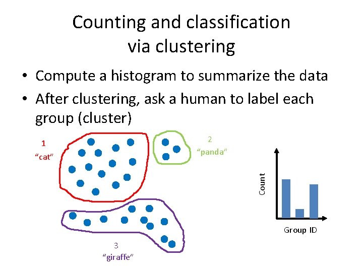
Counting and classification via clustering • Compute a histogram to summarize the data • After clustering, ask a human to label each group (cluster) 2 “panda” 1 Count “cat” Group ID 3 “giraffe”

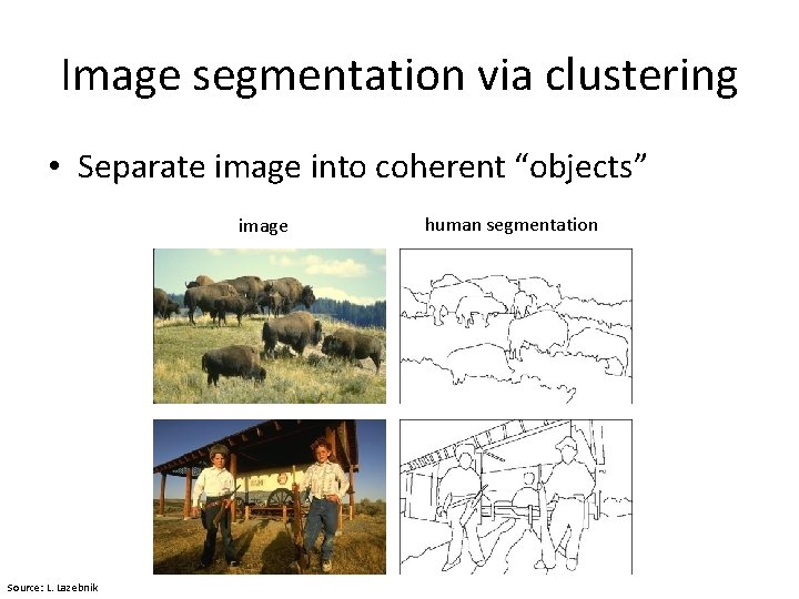
Image segmentation via clustering • Separate image into coherent “objects” image Source: L. Lazebnik human segmentation

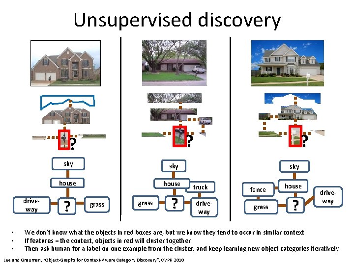
Unsupervised discovery ? ? driveway • • • sky house ? grass ? ? sky truck driveway fence grass house ? driveway We don’t know what the objects in red boxes are, but we know they tend to occur in similar context If features = the context, objects in red will cluster together Then ask human for a label on one example from the cluster, and keep learning new object categories iteratively Lee and Grauman, “Object-Graphs for Context-Aware Category Discovery”, CVPR 2010

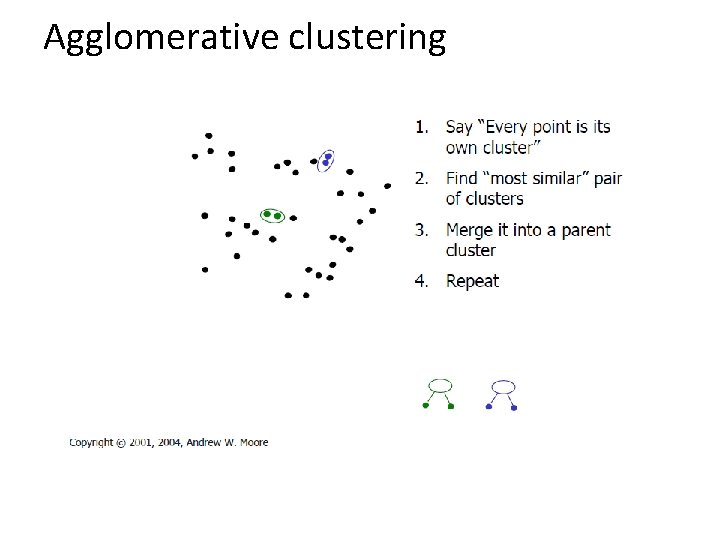
Today and next class • Clustering: motivation and applications • Algorithms – K-means (iterate between finding centers and assigning points) – Mean-shift (find modes in the data) – Hierarchical clustering (start with all points in separate clusters and merge) – Normalized cuts (split nodes in a graph based on similarity)

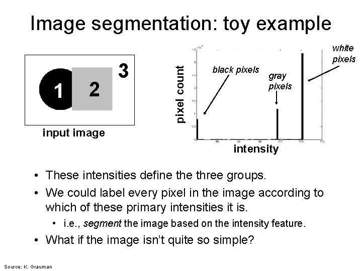
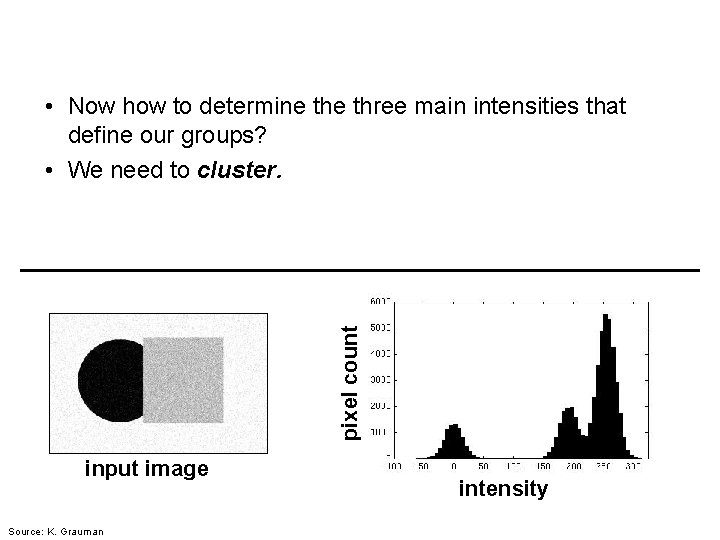
Image segmentation: toy example 2 pixel count 1 3 white pixels black pixels gray pixels input image intensity • These intensities define three groups. • We could label every pixel in the image according to which of these primary intensities it is. • i. e. , segment the image based on the intensity feature. • What if the image isn’t quite so simple? Source: K. Grauman

pixel count • Now how to determine three main intensities that define our groups? • We need to cluster. input image pixel count intensity input image Source: K. Grauman intensity

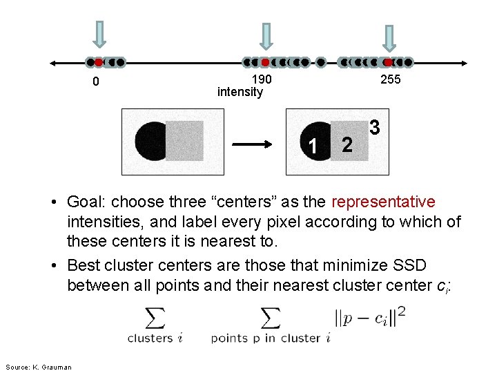
0 190 intensity 255 1 2 3 • Goal: choose three “centers” as the representative intensities, and label every pixel according to which of these centers it is nearest to. • Best cluster centers are those that minimize SSD between all points and their nearest cluster center ci: Source: K. Grauman

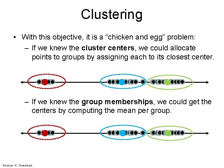
Clustering • With this objective, it is a “chicken and egg” problem: – If we knew the cluster centers, we could allocate points to groups by assigning each to its closest center. – If we knew the group memberships, we could get the centers by computing the mean per group. Source: K. Grauman

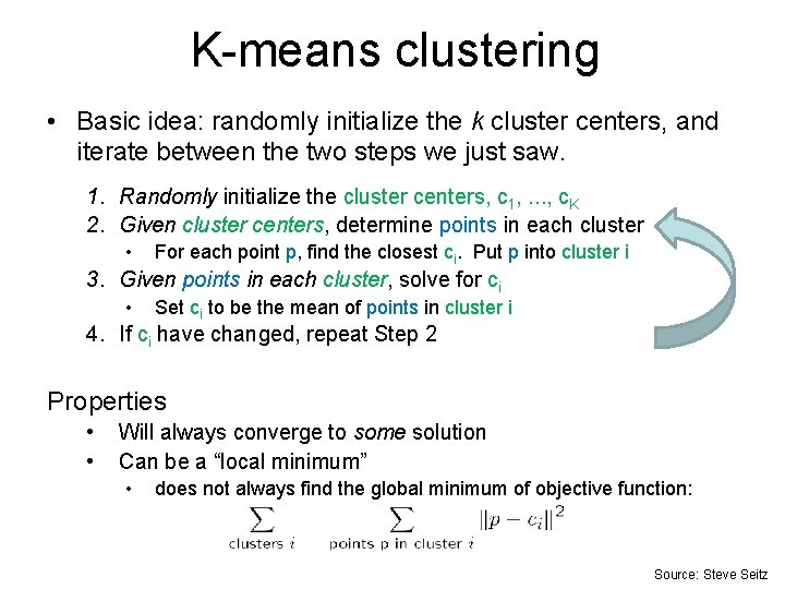
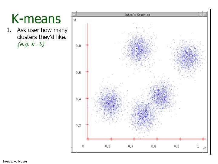
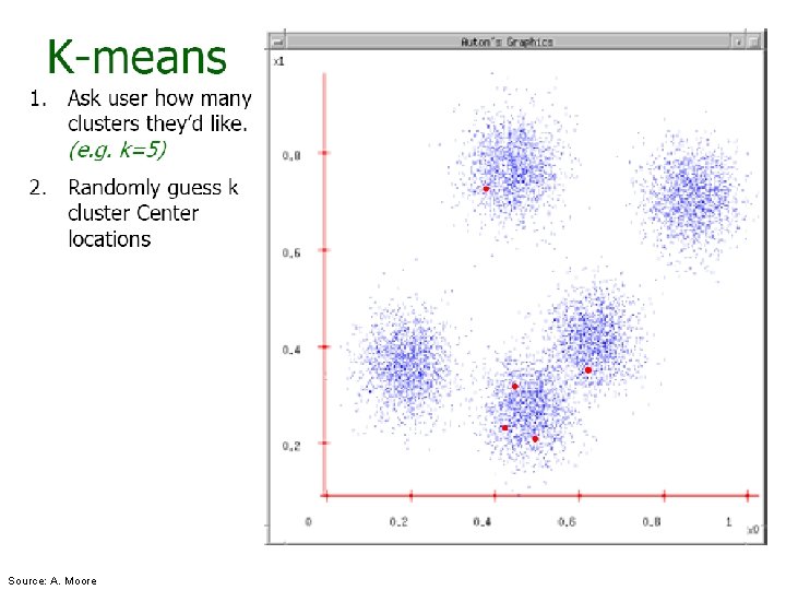
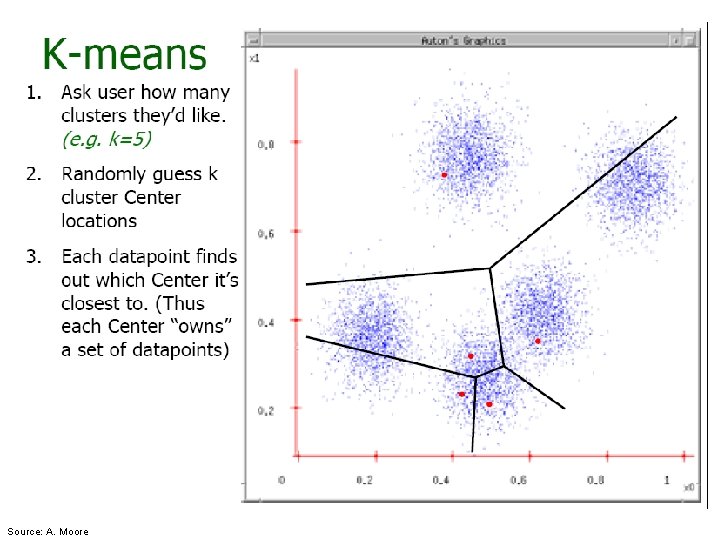
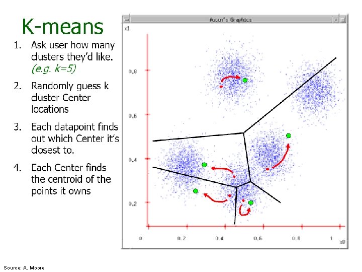
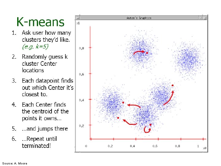
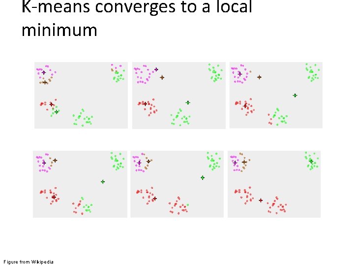
K-means clustering • Basic idea: randomly initialize the k cluster centers, and iterate between the two steps we just saw. 1. Randomly initialize the cluster centers, c 1, . . . , c. K 2. Given cluster centers, determine points in each cluster • For each point p, find the closest ci. Put p into cluster i 3. Given points in each cluster, solve for ci • Set ci to be the mean of points in cluster i 4. If ci have changed, repeat Step 2 Properties • • Will always converge to some solution Can be a “local minimum” • does not always find the global minimum of objective function: Source: Steve Seitz

Source: A. Moore

Source: A. Moore

Source: A. Moore

Source: A. Moore

Source: A. Moore

K-means converges to a local minimum Figure from Wikipedia

K-means clustering • Java demo http: //home. dei. polimi. it/matteucc/Clustering/tutoria l_html/Applet. KM. html • Matlab demo http: //www. cs. pitt. edu/~kovashka/cs 1699/kmeans_ demo. m

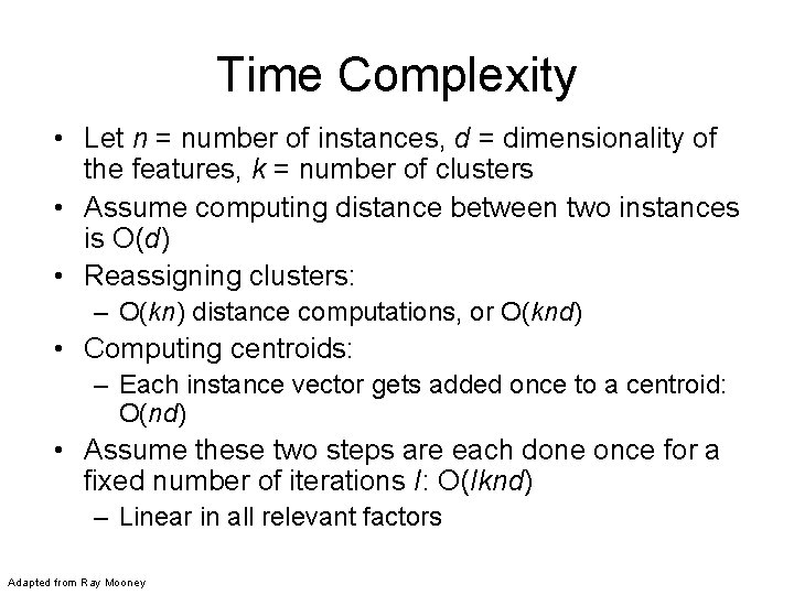
Time Complexity • Let n = number of instances, d = dimensionality of the features, k = number of clusters • Assume computing distance between two instances is O(d) • Reassigning clusters: – O(kn) distance computations, or O(knd) • Computing centroids: – Each instance vector gets added once to a centroid: O(nd) • Assume these two steps are each done once for a fixed number of iterations I: O(Iknd) – Linear in all relevant factors Adapted from Ray Mooney

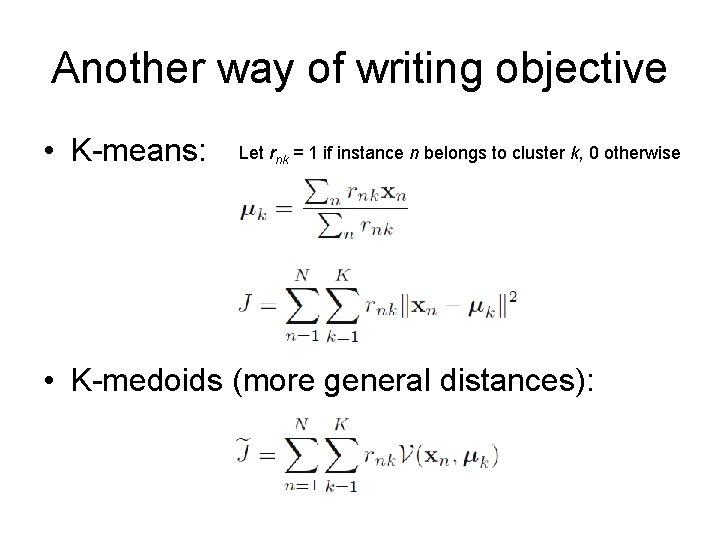
Another way of writing objective • K-means: Let rnk = 1 if instance n belongs to cluster k, 0 otherwise • K-medoids (more general distances):

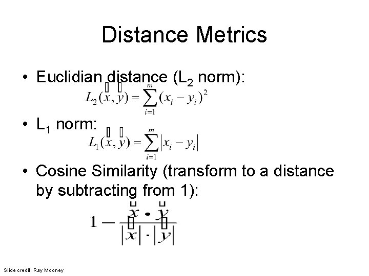
Distance Metrics • Euclidian distance (L 2 norm): • L 1 norm: • Cosine Similarity (transform to a distance by subtracting from 1): Slide credit: Ray Mooney

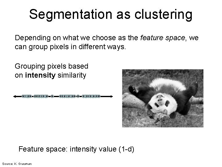
Segmentation as clustering Depending on what we choose as the feature space, we can group pixels in different ways. Grouping pixels based on intensity similarity Feature space: intensity value (1 -d) Source: K. Grauman

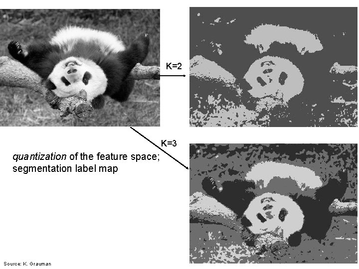
K=2 K=3 quantization of the feature space; segmentation label map Source: K. Grauman

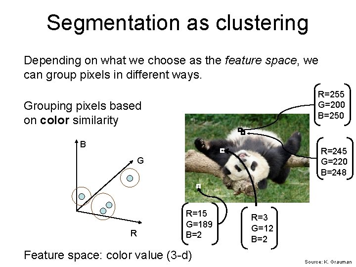
Segmentation as clustering Depending on what we choose as the feature space, we can group pixels in different ways. R=255 G=200 B=250 Grouping pixels based on color similarity B R=245 G=220 B=248 G R R=15 G=189 B=2 Feature space: color value (3 -d) R=3 G=12 B=2 Source: K. Grauman

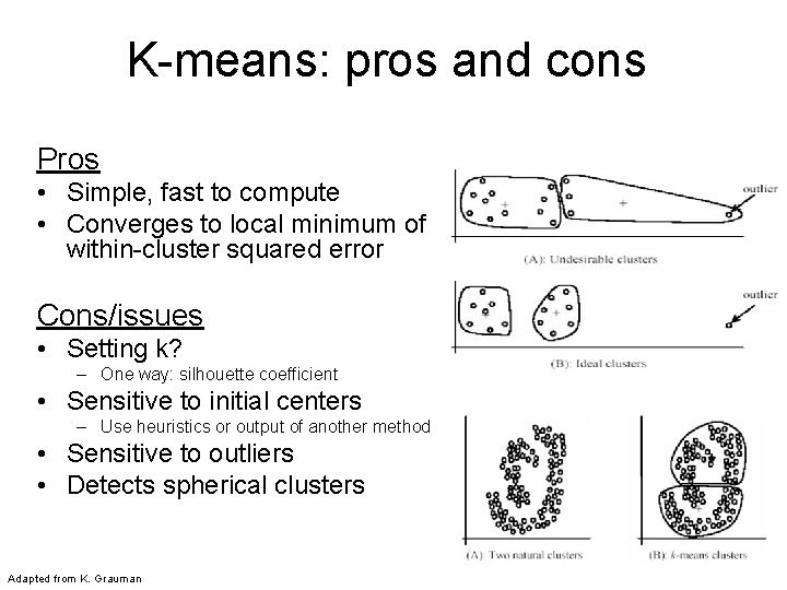
K-means: pros and cons Pros • Simple, fast to compute • Converges to local minimum of within-cluster squared error Cons/issues • Setting k? – One way: silhouette coefficient • Sensitive to initial centers – Use heuristics or output of another method • Sensitive to outliers • Detects spherical clusters Adapted from K. Grauman

Today • Clustering: motivation and applications • Algorithms – K-means (iterate between finding centers and assigning points) – Mean-shift (find modes in the data) – Hierarchical clustering (start with all points in separate clusters and merge) – Normalized cuts (split nodes in a graph based on similarity)

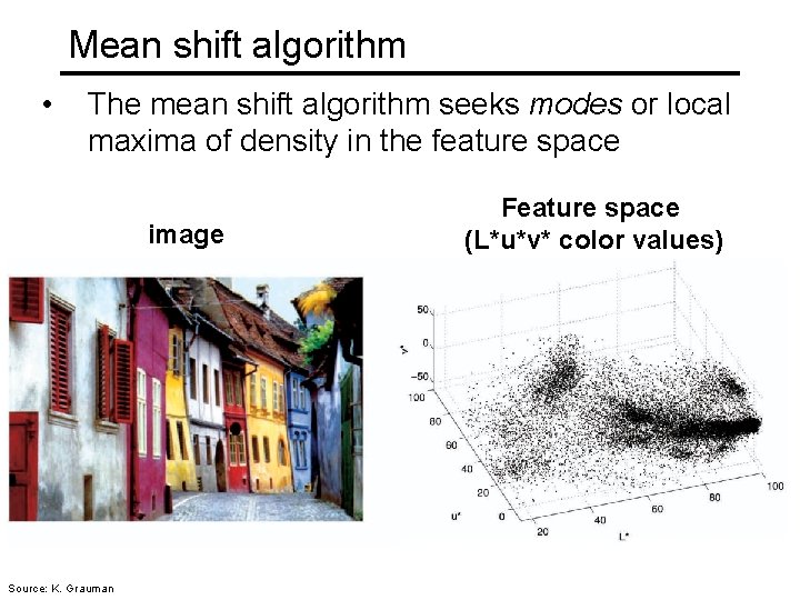
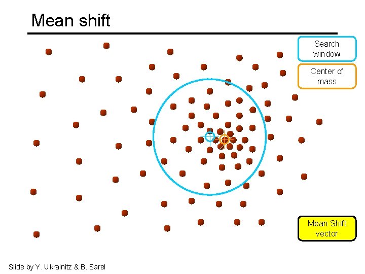
Mean shift algorithm • The mean shift algorithm seeks modes or local maxima of density in the feature space image Source: K. Grauman Feature space (L*u*v* color values)

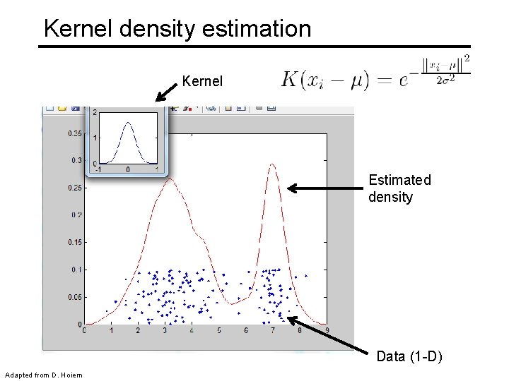
Kernel density estimation Kernel Estimated density Data (1 -D) Adapted from D. Hoiem

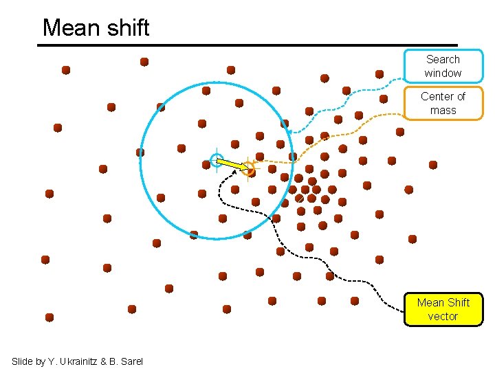
Mean shift Search window Center of mass Mean Shift vector Slide by Y. Ukrainitz & B. Sarel

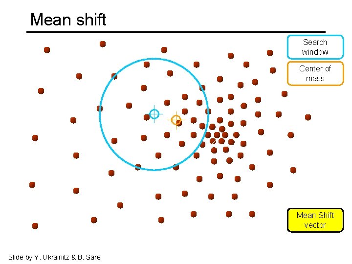
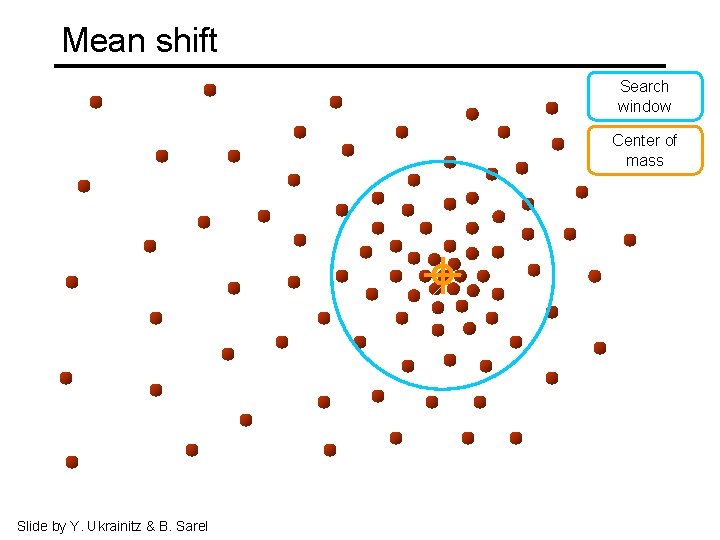
Mean shift Search window Center of mass Mean Shift vector Slide by Y. Ukrainitz & B. Sarel

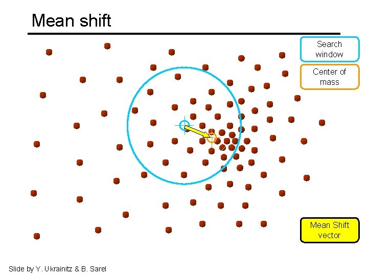
Mean shift Search window Center of mass Mean Shift vector Slide by Y. Ukrainitz & B. Sarel

Mean shift Search window Center of mass Mean Shift vector Slide by Y. Ukrainitz & B. Sarel

Mean shift Search window Center of mass Mean Shift vector Slide by Y. Ukrainitz & B. Sarel

Mean shift Search window Center of mass Mean Shift vector Slide by Y. Ukrainitz & B. Sarel

Mean shift Search window Center of mass Slide by Y. Ukrainitz & B. Sarel

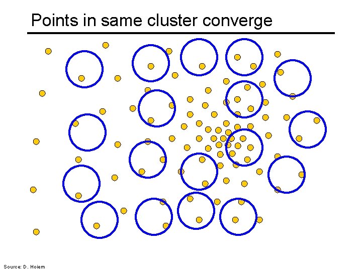
Points in same cluster converge Source: D. Hoiem

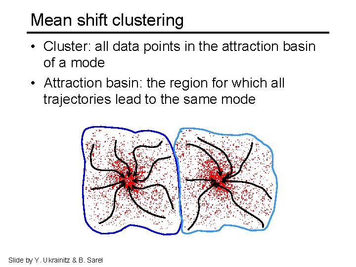
Mean shift clustering • Cluster: all data points in the attraction basin of a mode • Attraction basin: the region for which all trajectories lead to the same mode Slide by Y. Ukrainitz & B. Sarel

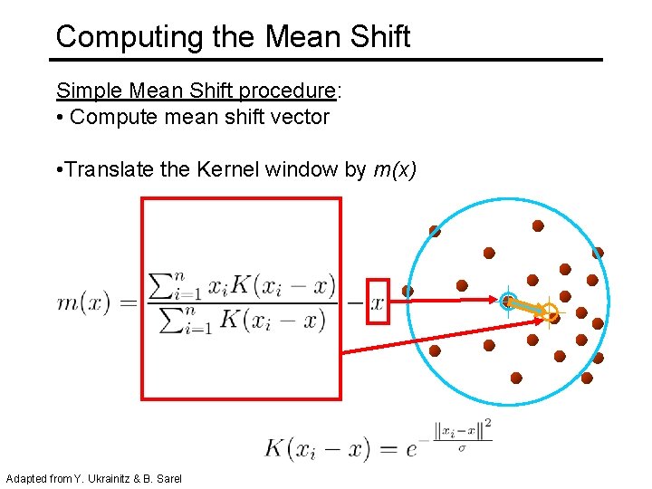
Computing the Mean Shift Simple Mean Shift procedure: • Compute mean shift vector • Translate the Kernel window by m(x) Adapted from Y. Ukrainitz & B. Sarel

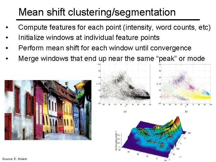
Mean shift clustering/segmentation • • Compute features for each point (intensity, word counts, etc) Initialize windows at individual feature points Perform mean shift for each window until convergence Merge windows that end up near the same “peak” or mode Source: D. Hoiem

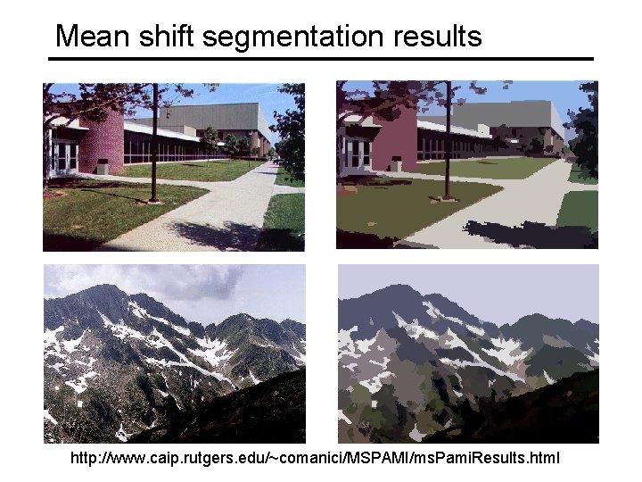
Mean shift segmentation results http: //www. caip. rutgers. edu/~comanici/MSPAMI/ms. Pami. Results. html

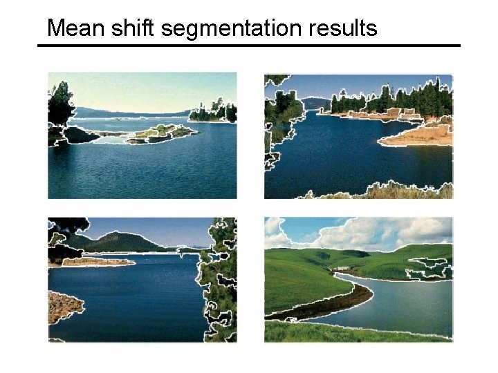
Mean shift segmentation results

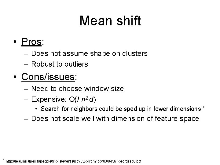
Mean shift • Pros: – Does not assume shape on clusters – Robust to outliers • Cons/issues: – Need to choose window size – Expensive: O(I n 2 d) • Search for neighbors could be sped up in lower dimensions * – Does not scale well with dimension of feature space * http: //lear. inrialpes. fr/people/triggs/events/iccv 03/cdrom/iccv 03/0456_georgescu. pdf

Mean-shift reading • Nicely written mean-shift explanation (with math) http: //saravananthirumuruganathan. wordpress. com/2010/04/01/introduction-to-mean-shiftalgorithm/ • Includes. m code for mean-shift clustering • Mean-shift paper by Comaniciu and Meer http: //citeseerx. ist. psu. edu/viewdoc/summary? doi=10. 1. 1. 76. 8968 • Adaptive mean shift in higher dimensions http: //lear. inrialpes. fr/people/triggs/events/iccv 03/cdrom/iccv 03/0456_georgescu. pdf https: //pdfs. semanticscholar. org/d 8 a 4/d 6 c 60 d 0 b 833 a 82 cd 92059891 a 6980 ff 54526. pdf Source: K. Grauman

Today • Clustering: motivation and applications • Algorithms – K-means (iterate between finding centers and assigning points) – Mean-shift (find modes in the data) – Hierarchical clustering (start with all points in separate clusters and merge) – Normalized cuts (split nodes in a graph based on similarity)

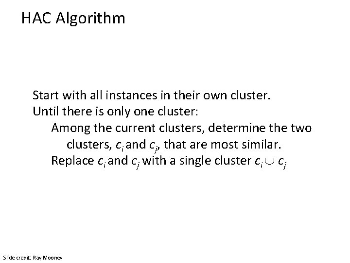
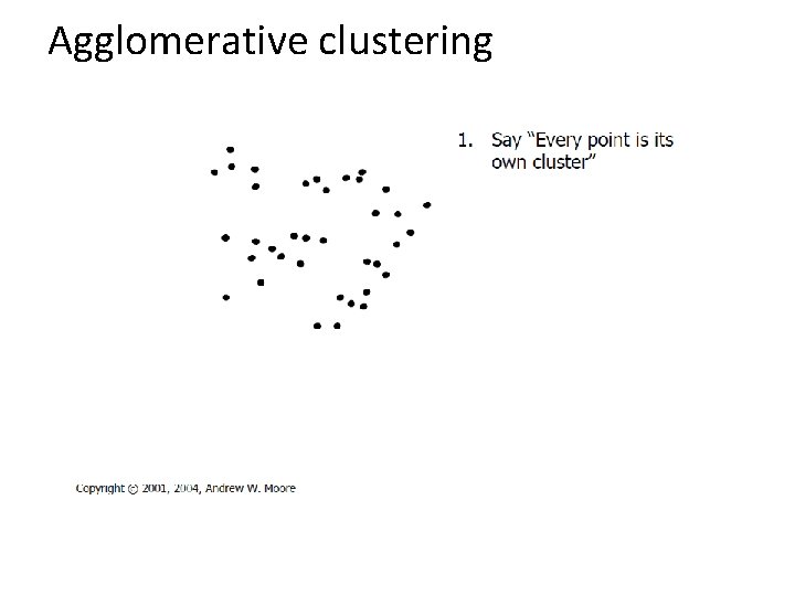
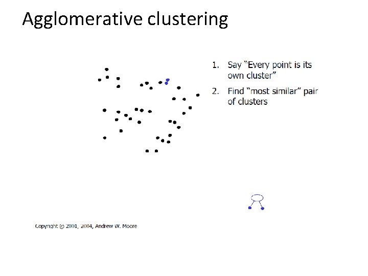
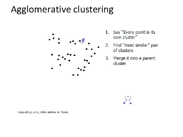
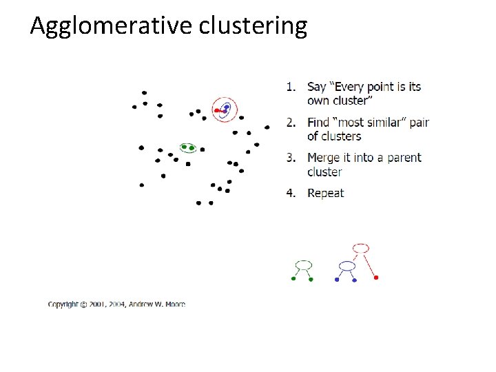
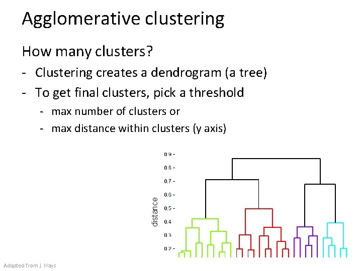
Hierarchical Agglomerative Clustering (HAC) • Assumes a similarity function for determining the similarity of two instances. • Starts with all instances in separate clusters and then repeatedly joins the two clusters that are most similar until there is only one cluster. • The history of merging forms a binary tree or hierarchy. Slide credit: Ray Mooney

HAC Algorithm Start with all instances in their own cluster. Until there is only one cluster: Among the current clusters, determine the two clusters, ci and cj, that are most similar. Replace ci and cj with a single cluster ci cj Slide credit: Ray Mooney

Agglomerative clustering

Agglomerative clustering

Agglomerative clustering

Agglomerative clustering

Agglomerative clustering

Agglomerative clustering How many clusters? - Clustering creates a dendrogram (a tree) - To get final clusters, pick a threshold distance - max number of clusters or - max distance within clusters (y axis) Adapted from J. Hays

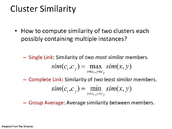
Cluster Similarity • How to compute similarity of two clusters each possibly containing multiple instances? – Single Link: Similarity of two most similar members. – Complete Link: Similarity of two least similar members. – Group Average: Average similarity between members. Adapted from Ray Mooney

Today • Clustering: motivation and applications • Algorithms – K-means (iterate between finding centers and assigning points) – Mean-shift (find modes in the data) – Hierarchical clustering (start with all points in separate clusters and merge) – Normalized cuts (split nodes in a graph based on similarity)

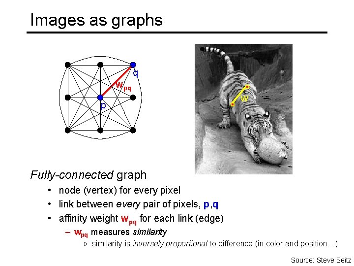
Images as graphs q wpq p w Fully-connected graph • node (vertex) for every pixel • link between every pair of pixels, p, q • affinity weight wpq for each link (edge) – wpq measures similarity » similarity is inversely proportional to difference (in color and position…) Source: Steve Seitz

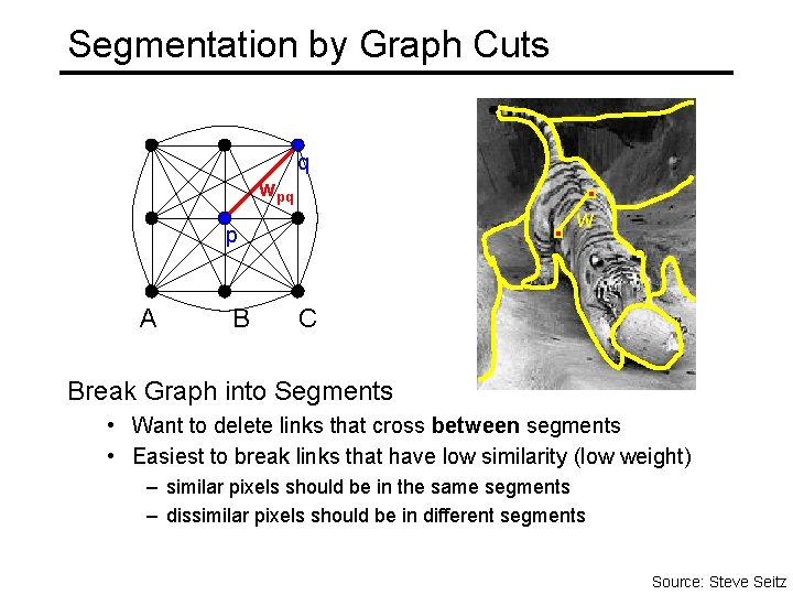
Segmentation by Graph Cuts q wpq w p A B C Break Graph into Segments • Want to delete links that cross between segments • Easiest to break links that have low similarity (low weight) – similar pixels should be in the same segments – dissimilar pixels should be in different segments Source: Steve Seitz

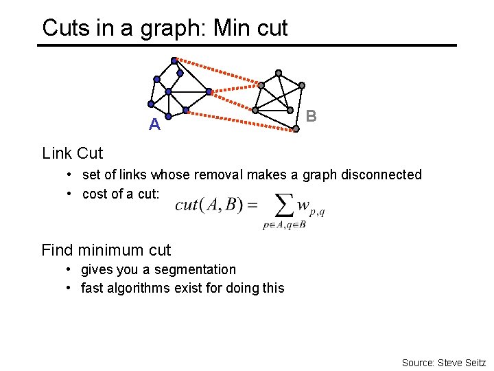
Cuts in a graph: Min cut A B Link Cut • set of links whose removal makes a graph disconnected • cost of a cut: Find minimum cut • gives you a segmentation • fast algorithms exist for doing this Source: Steve Seitz

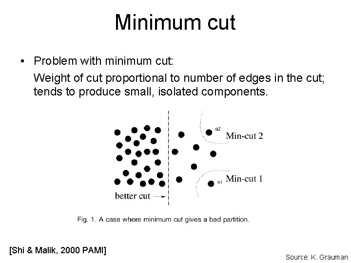
Minimum cut • Problem with minimum cut: Weight of cut proportional to number of edges in the cut; tends to produce small, isolated components. [Shi & Malik, 2000 PAMI] Source: K. Grauman

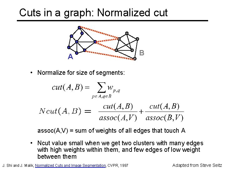
Cuts in a graph: Normalized cut A B • Normalize for size of segments: assoc(A, V) = sum of weights of all edges that touch A • Ncut value small when we get two clusters with many edges with high weights within them, and few edges of low weight between them J. Shi and J. Malik, Normalized Cuts and Image Segmentation, CVPR, 1997 Adapted from Steve Seitz

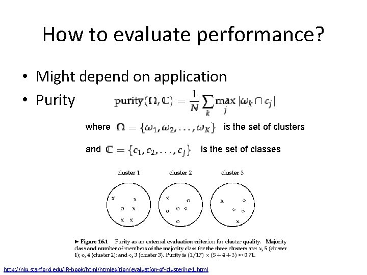
How to evaluate performance? • Might depend on application • Purity is the set of clusters where and is the set of classes http: //nlp. stanford. edu/IR-book/htmledition/evaluation-of-clustering-1. html

How to evaluate performance • See Murphy Sec. 25. 1 for another two metrics (Rand index and mutual information)

Clustering Strategies • K-means – Iteratively re-assign points to the nearest cluster center • Mean-shift clustering – Estimate modes • Graph cuts – Split the nodes in a graph based on assigned links with similarity weights • Agglomerative clustering – Start with each point as its own cluster and iteratively merge the closest clusters