CS 2750 Machine Learning Expectation Maximization Prof Adriana

CS 2750: Machine Learning Expectation Maximization Prof. Adriana Kovashka University of Pittsburgh April 11, 2017

Plan for this lecture • • • EM for Hidden Markov Models (last lecture) EM for Gaussian Mixture Models EM in general K-means ~ GMM EM for Naïve Bayes

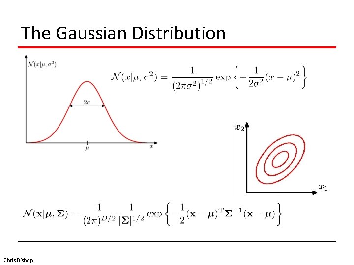
The Gaussian Distribution Chris Bishop

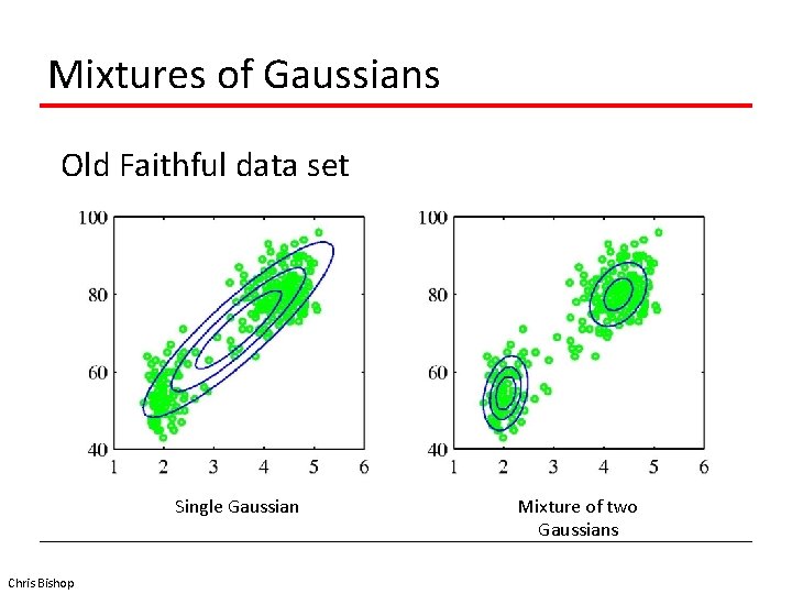
Mixtures of Gaussians Old Faithful data set Single Gaussian Chris Bishop Mixture of two Gaussians

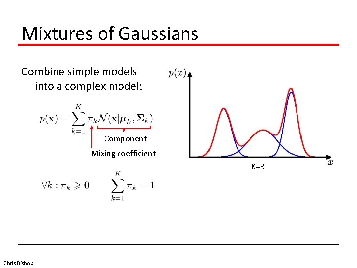
Mixtures of Gaussians Combine simple models into a complex model: Component Mixing coefficient K=3 Chris Bishop

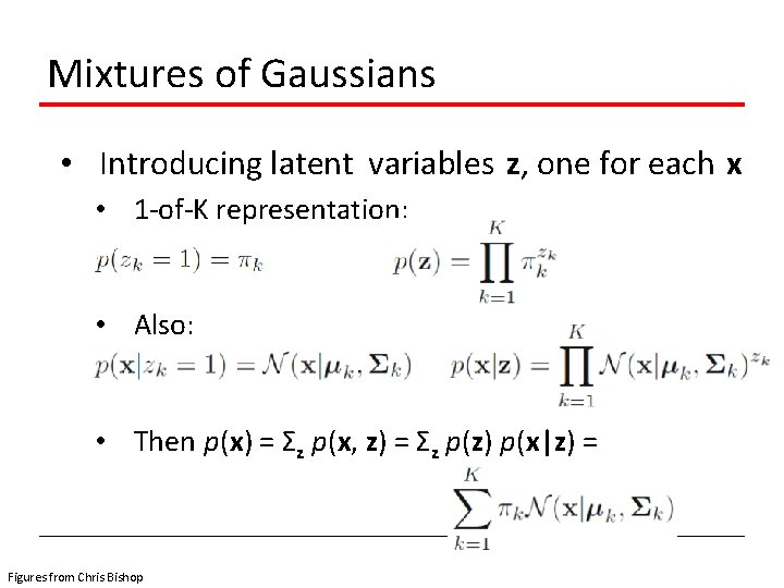
Mixtures of Gaussians • Introducing latent variables z, one for each x • 1 -of-K representation: • Also: • Then p(x) = Σz p(x, z) = Σz p(z) p(x|z) = Figures from Chris Bishop

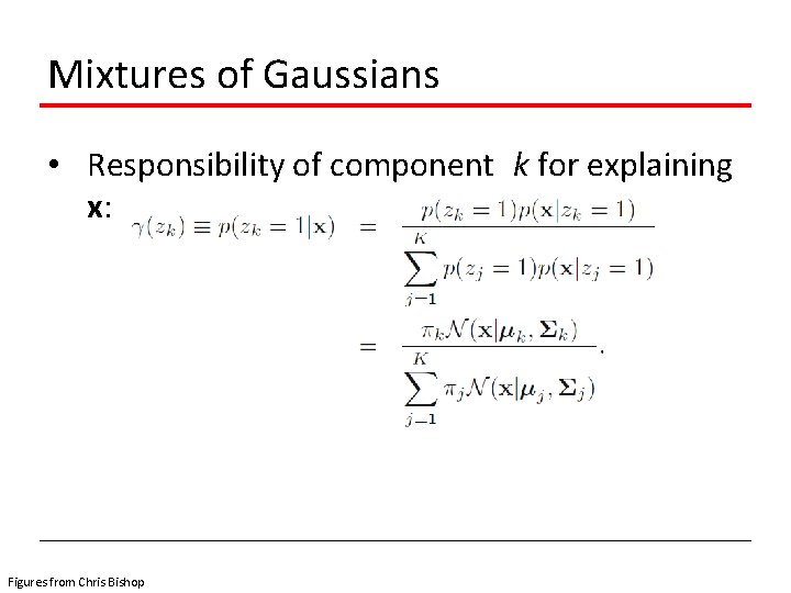
Mixtures of Gaussians • Responsibility of component k for explaining x: Figures from Chris Bishop

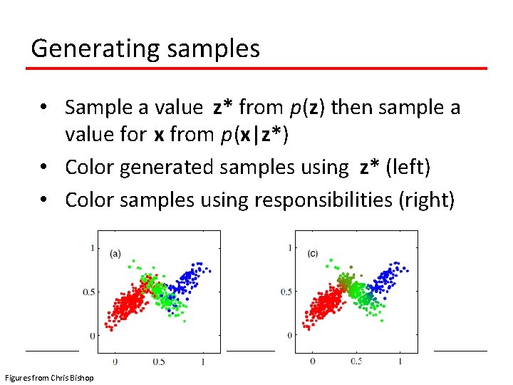
Generating samples • Sample a value z* from p(z) then sample a value for x from p(x|z*) • Color generated samples using z* (left) • Color samples using responsibilities (right) Figures from Chris Bishop

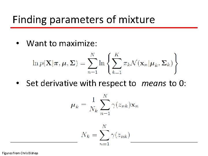
Finding parameters of mixture • Want to maximize: • Set derivative with respect to means to 0: Figures from Chris Bishop

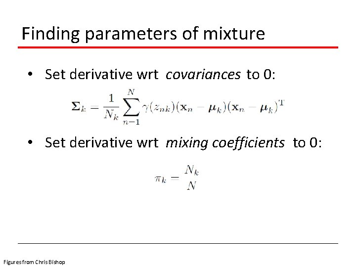
Finding parameters of mixture • Set derivative wrt covariances to 0: • Set derivative wrt mixing coefficients to 0: Figures from Chris Bishop

Reminder • Responsibilities: • So parameters of GMM depend on responsibilities and vice versa… • What can we do? Figures from Chris Bishop

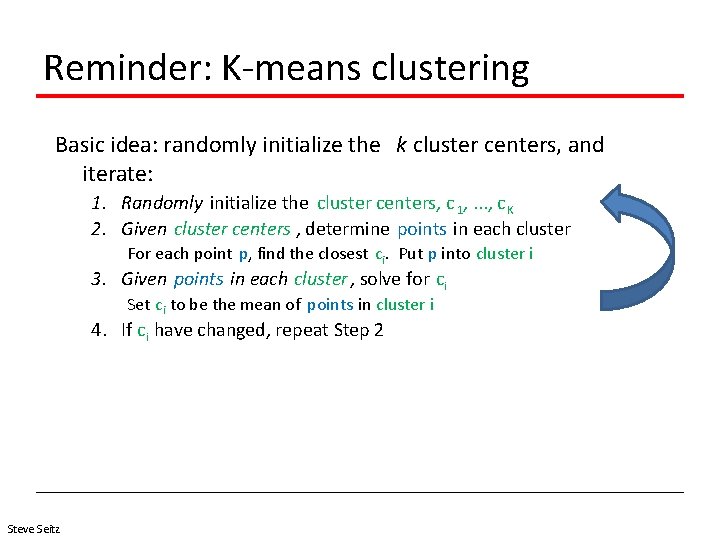
Reminder: K-means clustering Basic idea: randomly initialize the k cluster centers, and iterate: 1. Randomly initialize the cluster centers, c 1, . . . , c K 2. Given cluster centers , determine points in each cluster For each point p, find the closest ci. Put p into cluster i 3. Given points in each cluster , solve for ci Set ci to be the mean of points in cluster i 4. If ci have changed, repeat Step 2 Steve Seitz

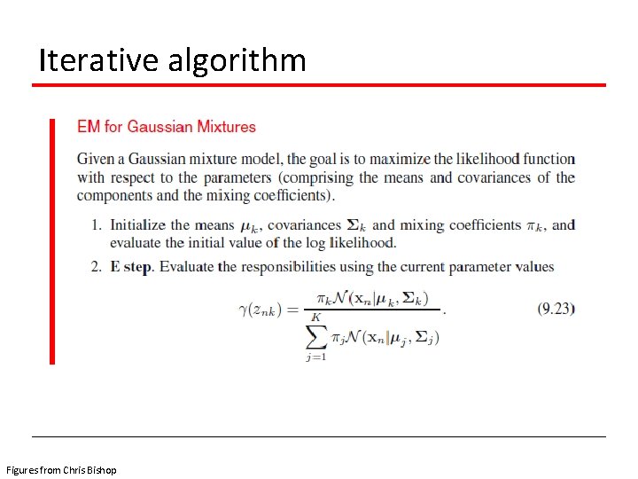
Iterative algorithm Figures from Chris Bishop

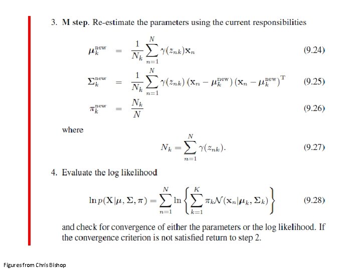
Figures from Chris Bishop

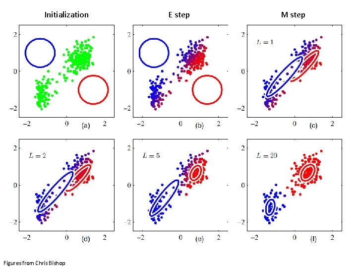
Initialization Figures from Chris Bishop E step M step

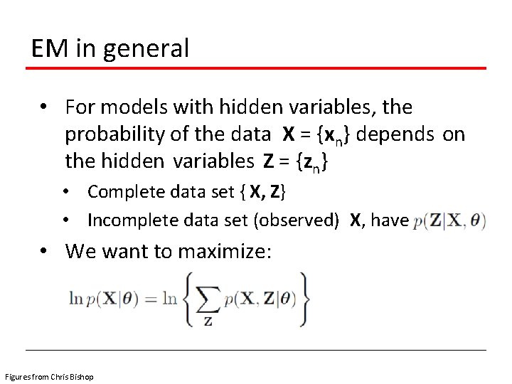
EM in general • For models with hidden variables, the probability of the data X = {xn} depends on the hidden variables Z = {zn} • Complete data set { X, Z} • Incomplete data set (observed) X, have • We want to maximize: Figures from Chris Bishop

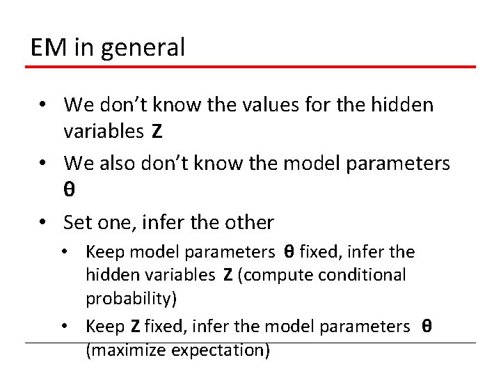
EM in general • We don’t know the values for the hidden variables Z • We also don’t know the model parameters θ • Set one, infer the other • Keep model parameters θ fixed, infer the hidden variables Z (compute conditional probability) • Keep Z fixed, infer the model parameters θ (maximize expectation)

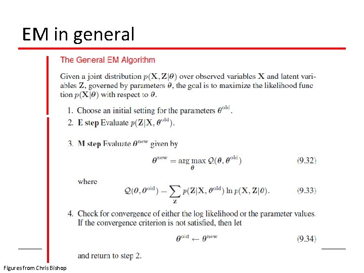
EM in general Figures from Chris Bishop

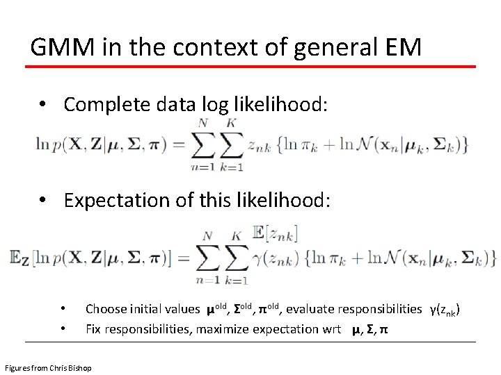
GMM in the context of general EM • Complete data log likelihood: • Expectation of this likelihood: • • Choose initial values μold, Σold, πold, evaluate responsibilities γ(znk) Fix responsibilities, maximize expectation wrt μ, Σ, π Figures from Chris Bishop

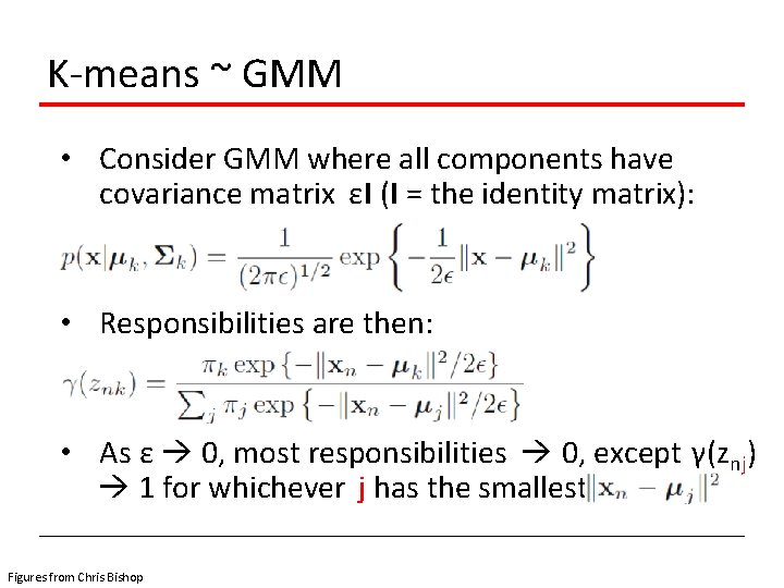
K-means ~ GMM • Consider GMM where all components have covariance matrix εI (I = the identity matrix): • Responsibilities are then: • As ε 0, most responsibilities 0, except γ(znj) 1 for whichever j has the smallest Figures from Chris Bishop

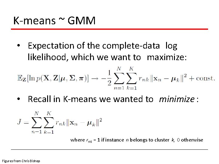
K-means ~ GMM • Expectation of the complete-data log likelihood, which we want to maximize: • Recall in K-means we wanted to minimize : where rnk = 1 if instance n belongs to cluster k, 0 otherwise Figures from Chris Bishop

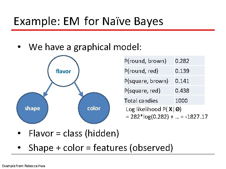
Example: EM for Naïve Bayes • We have a graphical model: flavor shape color P(round, brown) 0. 282 P(round, red) 0. 139 P(square, brown) 0. 141 P(square, red) 0. 438 Total candies 1000 Log likelihood P( X|Θ) = 282*log(0. 282) + … = -1827. 17 • Flavor = class (hidden) • Shape + color = features (observed) Example from Rebecca Hwa

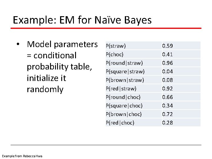
Example: EM for Naïve Bayes • Model parameters = conditional probability table, initialize it randomly Example from Rebecca Hwa P(straw) P(choc) P(round|straw) P(square|straw) P(brown|straw) P(red|straw) P(round|choc) P(square|choc) P(brown|choc) P(red|choc) 0. 59 0. 41 0. 96 0. 04 0. 08 0. 92 0. 66 0. 34 0. 72 0. 28

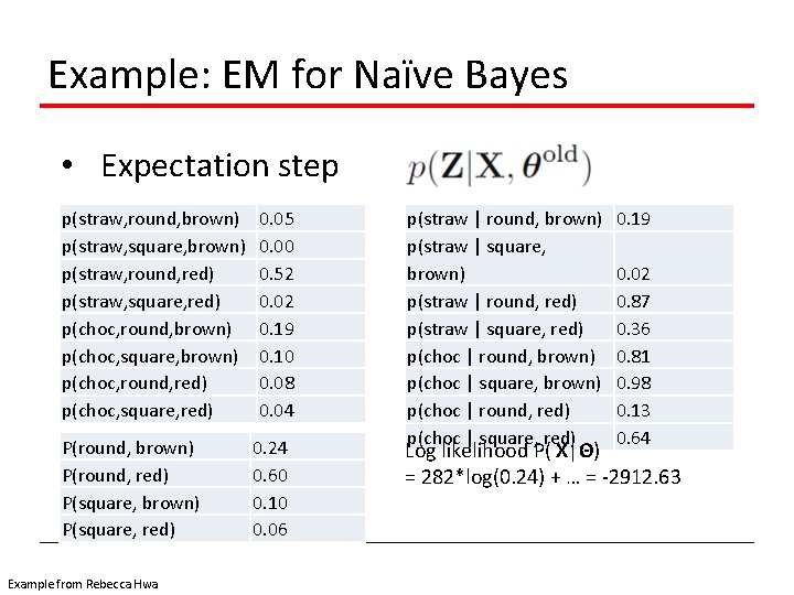
Example: EM for Naïve Bayes • Expectation step • Keeping model (CPT) fixed, estimate values for joint probability distribution by multiplying P(flavor) * P(shape|flavor) * P(color|flavor) • Then use these to compute conditional probability of the hidden variable flavor: P(straw|shape, color) = P(straw, shape, color) / P(shape, color ) = P(straw, shape, color) / Σflavor P(flavor, shape, color) Example from Rebecca Hwa

Example: EM for Naïve Bayes • Expectation step p(straw, round, brown) p(straw, square, brown) p(straw, round, red) p(straw, square, red) p(choc, round, brown) p(choc, square, brown) p(choc, round, red) p(choc, square, red) P(round, brown) P(round, red) P(square, brown) P(square, red) Example from Rebecca Hwa 0. 05 0. 00 0. 52 0. 02 0. 19 0. 10 0. 08 0. 04 0. 24 0. 60 0. 10 0. 06 p(straw | round, brown) p(straw | square, brown) p(straw | round, red) p(straw | square, red) p(choc | round, brown) p(choc | square, brown) p(choc | round, red) p(choc | square, red) 0. 19 0. 02 0. 87 0. 36 0. 81 0. 98 0. 13 0. 64 Log likelihood P( X|Θ) = 282*log(0. 24) + … = -2912. 63

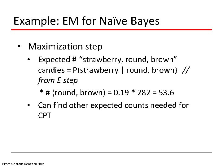
Example: EM for Naïve Bayes • Maximization step • Expected # “strawberry, round, brown” candies = P(strawberry | round, brown) // from E step * # (round, brown) = 0. 19 * 282 = 53. 6 • Can find other expected counts needed for CPT Example from Rebecca Hwa

Example: EM for Naïve Bayes • Maximization step exp # straw, round exp. # straw, square exp # straw, red exp # straw, brown exp # straw exp # choc, round exp # choc, square exp # choc, red exp # choc, brown exp # choc Example from Rebecca Hwa 174. 56 159. 16 277. 91 55. 81 333. 72 246. 44 419. 84 299. 09 367. 19 666. 28 P(straw) P(choc) P(round|straw) P(square|straw) P(brown|straw) P(red|straw) P(round|choc) P(square|choc) P(brown|choc) P(red|choc) 0. 33 0. 67 0. 52 0. 48 0. 17 0. 83 0. 37 0. 63 0. 55 0. 45

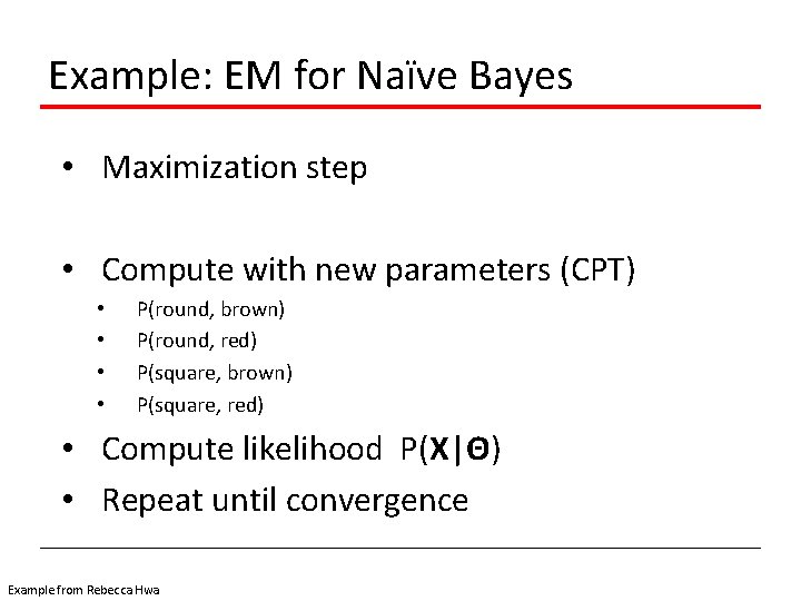
Example: EM for Naïve Bayes • Maximization step • Compute with new parameters (CPT) • • P(round, brown) P(round, red) P(square, brown) P(square, red) • Compute likelihood P(X|Θ) • Repeat until convergence Example from Rebecca Hwa