CS 15 346 Perspectives in Computer Architecture Pipelining

CS 15 -346 Perspectives in Computer Architecture Pipelining and Instruction Level Parallelism Lecture 6 January 30 th, 2013

Objectives • Origins of computing concepts, from Pascal to Turing and von Neumann. • Principles and concepts of computer architectures in 20 th and 21 st centuries. • Basic architectural techniques including instruction level parallelism, pipelining, cache memories and multicore architectures • Architecture including various kinds of computers from largest and fastest to tiny and digestible. • New architectural requirements far beyond raw performance such as energy, programmability, security, and availability. • Architectures for mobile computing including considerations affecting hardware, systems, and end-to-end applications.

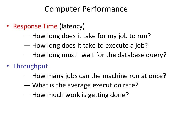
Computer Performance • Response Time (latency) — How long does it take for my job to run? — How long does it take to execute a job? — How long must I wait for the database query? • Throughput — How many jobs can the machine run at once? — What is the average execution rate? — How much work is getting done?

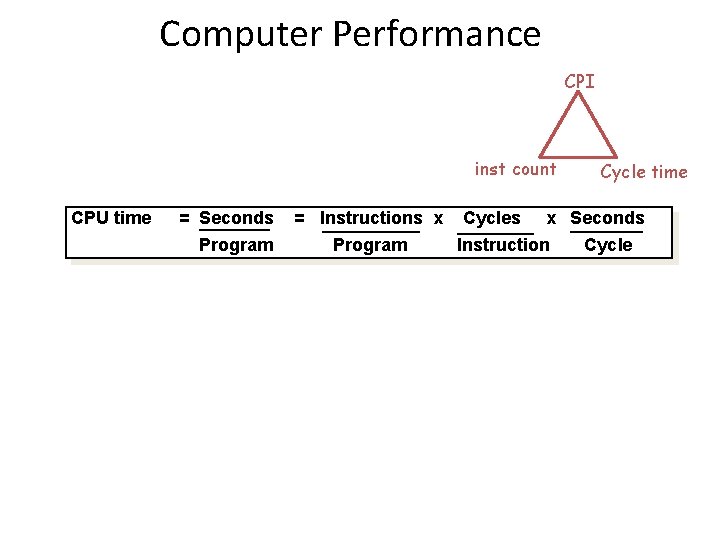
Computer Performance CPI inst count CPU time = Seconds Program = Instructions x Program Cycles Cycle time x Seconds Instruction Cycle

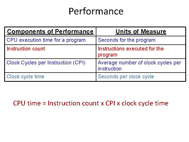
Performance Components of Performance Units of Measure CPU execution time for a program Seconds for the program Instruction count Instructions executed for the program Clock Cycles per Instruction (CPI) Average number of clock cycles per instruction Clock cycle time Seconds per clock cycle CPU time = Instruction count x CPI x clock cycle time

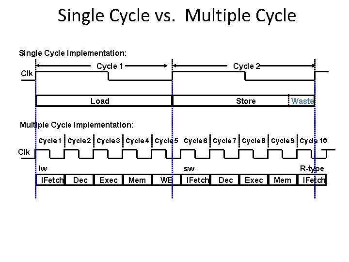
Single Cycle vs. Multiple Cycle Single Cycle Implementation: Cycle 1 Clk Cycle 2 Load Store Waste Multiple Cycle Implementation: Cycle 1 Cycle 2 Cycle 3 Cycle 4 Cycle 5 Cycle 6 Cycle 7 Cycle 8 Cycle 9 Cycle 10 Clk lw IFetch Dec Exec Mem WB sw IFetch Dec Exec Mem R-type IFetch

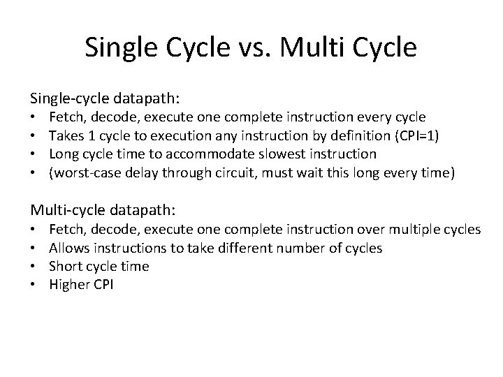
Single Cycle vs. Multi Cycle Single-cycle datapath: • • Fetch, decode, execute one complete instruction every cycle Takes 1 cycle to execution any instruction by definition (CPI=1) Long cycle time to accommodate slowest instruction (worst-case delay through circuit, must wait this long every time) Multi-cycle datapath: • • Fetch, decode, execute one complete instruction over multiple cycles Allows instructions to take different number of cycles Short cycle time Higher CPI

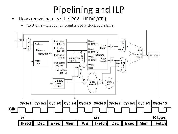
Pipelining and ILP • How can we increase the IPC? (IPC=1/CPI) – CPU time = Instruction count x CPI x clock cycle time Cycle 1 Cycle 2 Cycle 3 Cycle 4 Cycle 5 Cycle 6 Cycle 7 Cycle 8 Cycle 9 Cycle 10 Clk lw IFetch Dec Exec Mem WB sw IFetch Dec Exec Mem R-type IFetch

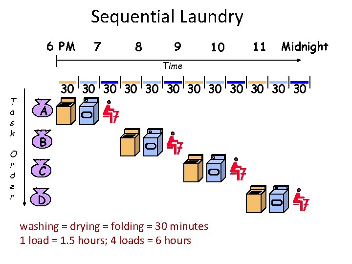
Sequential Laundry 6 PM 7 8 9 10 11 Midnight Time T a s k O r d e r 30 30 30 A B C D washing = drying = folding = 30 minutes 1 load = 1. 5 hours; 4 loads = 6 hours

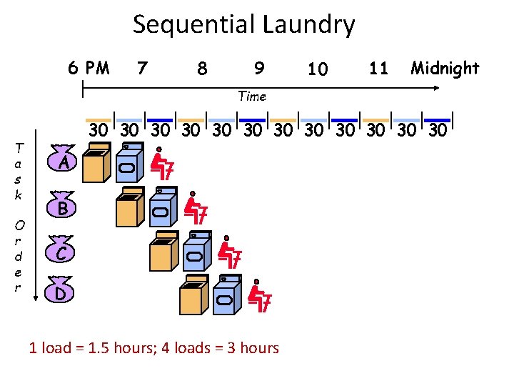
Sequential Laundry 6 PM 7 8 9 10 11 Midnight Time T a s k O r d e r 30 30 30 A B C D 1 load = 1. 5 hours; 4 loads = 3 hours

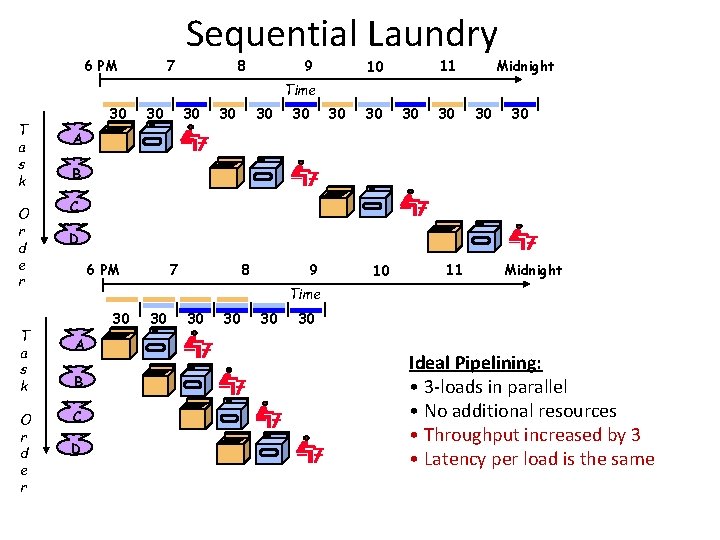
6 PM 7 Sequential Laundry 8 9 Midnight 11 10 Time T a s k O r d e r 30 30 30 A B C D 6 PM 7 8 9 10 11 Midnight Time 30 A B C D 30 30 30 Ideal Pipelining: • 3 -loads in parallel • No additional resources • Throughput increased by 3 • Latency per load is the same

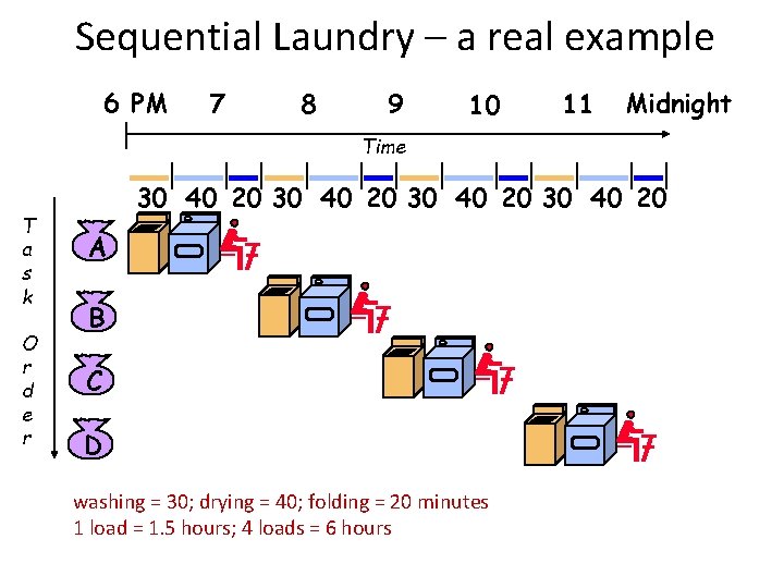
Sequential Laundry – a real example 6 PM 7 8 9 10 11 Midnight Time T a s k O r d e r 30 40 20 A B C D washing = 30; drying = 40; folding = 20 minutes 1 load = 1. 5 hours; 4 loads = 6 hours

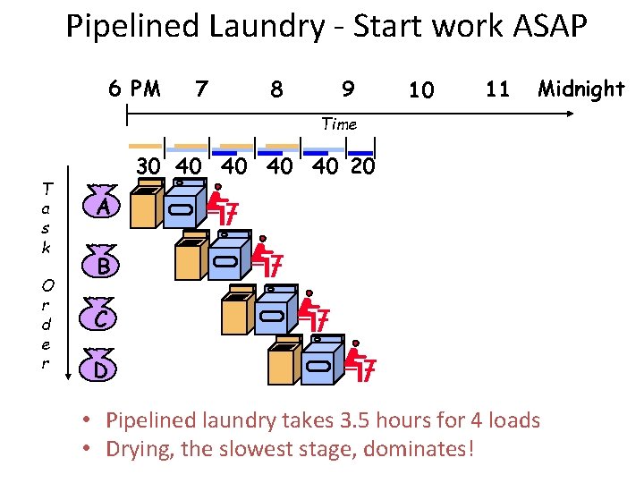
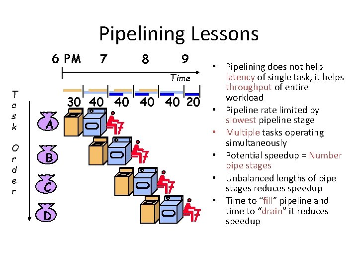
Pipelined Laundry - Start work ASAP 6 PM 7 8 9 10 11 Midnight Time T a s k O r d e r 30 40 40 20 A B C D • Pipelined laundry takes 3. 5 hours for 4 loads • Drying, the slowest stage, dominates!

Pipelining Lessons 6 PM 7 8 9 Time T a s k O r d e r 30 40 40 20 A B C D • Pipelining does not help latency of single task, it helps throughput of entire workload • Pipeline rate limited by slowest pipeline stage • Multiple tasks operating simultaneously • Potential speedup = Number pipe stages • Unbalanced lengths of pipe stages reduces speedup • Time to “fill” pipeline and time to “drain” it reduces speedup

Pipelining • Does not improve latency! • Programs execute billions of instructions, so throughput is what matters!

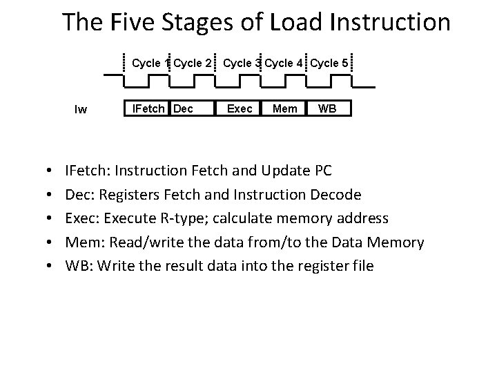
The Five Stages of Load Instruction Cycle 1 Cycle 2 Cycle 3 Cycle 4 Cycle 5 lw • • • IFetch Dec Exec Mem WB IFetch: Instruction Fetch and Update PC Dec: Registers Fetch and Instruction Decode Exec: Execute R-type; calculate memory address Mem: Read/write the data from/to the Data Memory WB: Write the result data into the register file

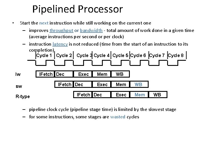
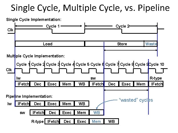
Pipelined Processor • Start the next instruction while still working on the current one – improves throughput or bandwidth - total amount of work done in a given time (average instructions per second or per clock) – instruction latency is not reduced (time from the start of an instruction to its completion) Cycle 1 Cycle 2 Cycle 3 Cycle 4 Cycle 5 Cycle 6 Cycle 7 Cycle 8 IFetch Dec lw Exec IFetch Dec sw R-type Mem WB Exec Mem IFetch Dec WB – pipeline clock cycle (pipeline stage time) is limited by the slowest stage – for some instructions, some stages are wasted cycles

Single Cycle, Multiple Cycle, vs. Pipeline Single Cycle Implementation: Cycle 1 Clk Cycle 2 Load Store Waste Multiple Cycle Implementation: Cycle 1 Cycle 2 Cycle 3 Cycle 4 Cycle 5 Cycle 6 Cycle 7 Cycle 8 Cycle 9 Cycle 10 Clk lw IFetch Dec Exec Mem WB sw IFetch Dec Pipeline Implementation: lw IFetch sw Mem “wasted” cycles Dec Exec Mem WB IFetch Dec Exec Mem WB Dec Exec Mem R-type IFetch Exec R-type IFetch WB

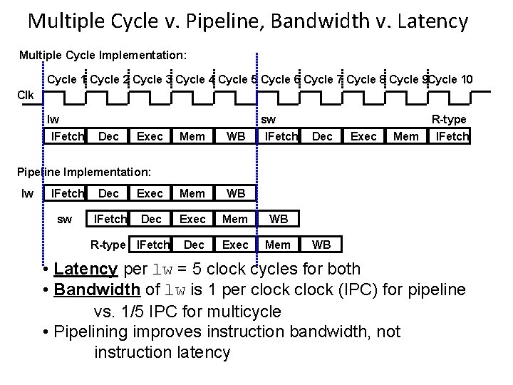
Multiple Cycle v. Pipeline, Bandwidth v. Latency Multiple Cycle Implementation: Cycle 1 Cycle 2 Cycle 3 Cycle 4 Cycle 5 Cycle 6 Cycle 7 Cycle 8 Cycle 9 Cycle 10 Clk lw IFetch Dec Exec Mem WB sw IFetch Dec Exec Mem R-type IFetch Pipeline Implementation: lw IFetch sw Dec Exec Mem WB IFetch Dec Exec Mem WB Dec Exec Mem R-type IFetch WB • Latency per lw = 5 clock cycles for both • Bandwidth of lw is 1 per clock (IPC) for pipeline vs. 1/5 IPC for multicycle • Pipelining improves instruction bandwidth, not instruction latency

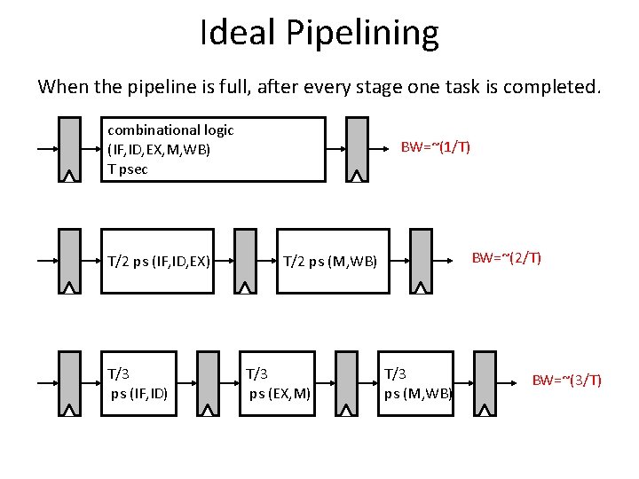
Ideal Pipelining When the pipeline is full, after every stage one task is completed. combinational logic (IF, ID, EX, M, WB) T psec T/2 ps (IF, ID, EX) T/3 ps (IF, ID) BW=~(1/T) BW=~(2/T) T/2 ps (M, WB) T/3 ps (EX, M) T/3 ps (M, WB) BW=~(3/T)

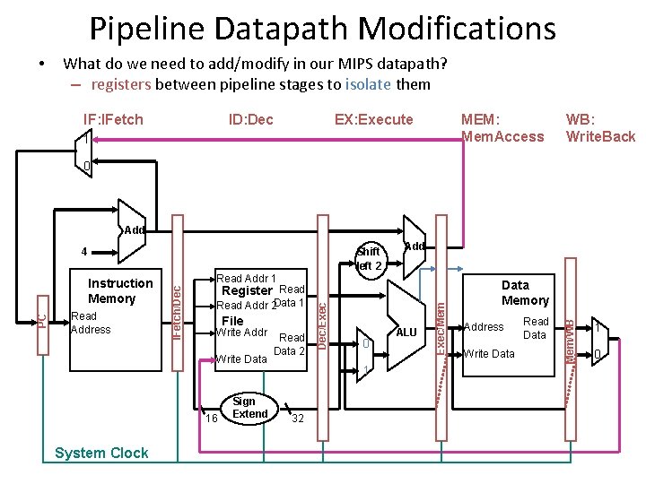
Pipeline Datapath Modifications • What do we need to add/modify in our MIPS datapath? – registers between pipeline stages to isolate them IF: IFetch ID: Dec EX: Execute MEM: Mem. Access 1 WB: Write. Back 0 Add Read Addr 2 Data 1 File Write Addr Write Data 16 System Clock Sign Extend Read Data 2 0 1 32 ALU Exec/Mem Register Read Dec/Exec Read Address Read Addr 1 IFetch/Dec PC Instruction Memory Add Data Memory Address Write Data Read Data Mem/WB Shift left 2 4 1 0

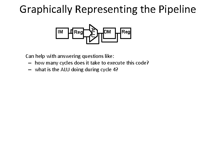
Graphically Representing the Pipeline Reg ALU IM DM Reg Can help with answering questions like: – how many cycles does it take to execute this code? – what is the ALU doing during cycle 4?

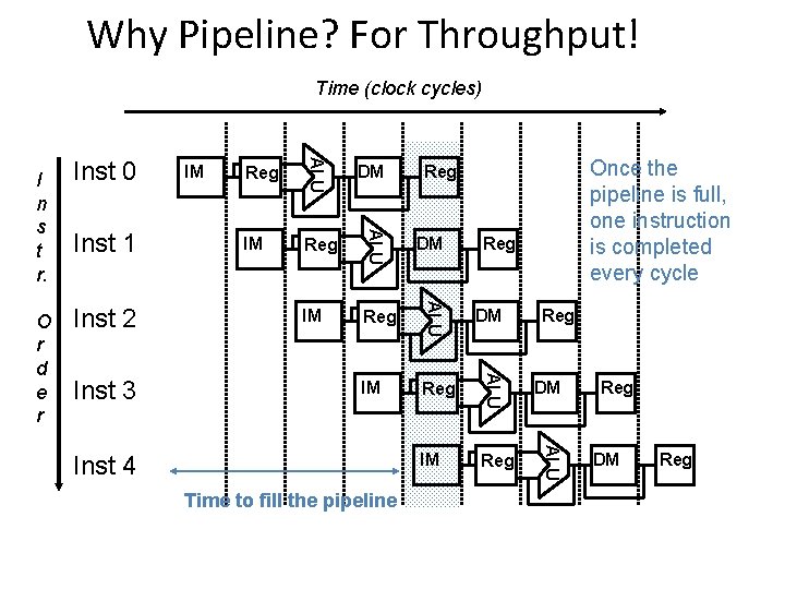
Why Pipeline? For Throughput! Time (clock cycles) IM Reg DM IM Reg ALU Inst 3 DM ALU Inst 2 Once the pipeline is full, one instruction is completed every cycle Reg ALU Inst 1 IM ALU O r d e r Inst 0 ALU I n s t r. Inst 4 Time to fill the pipeline Reg Reg DM Reg

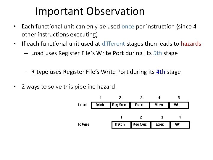
Important Observation • Each functional unit can only be used once per instruction (since 4 other instructions executing) • If each functional unit used at different stages then leads to hazards: – Load uses Register File’s Write Port during its 5 th stage – R-type uses Register File’s Write Port during its 4 th stage • 2 ways to solve this pipeline hazard. 1 Load Ifetch 2 Reg/Dec 1 R-type Ifetch 3 Exec 2 Reg/Dec 4 5 Mem Wr 3 4 Exec Wr

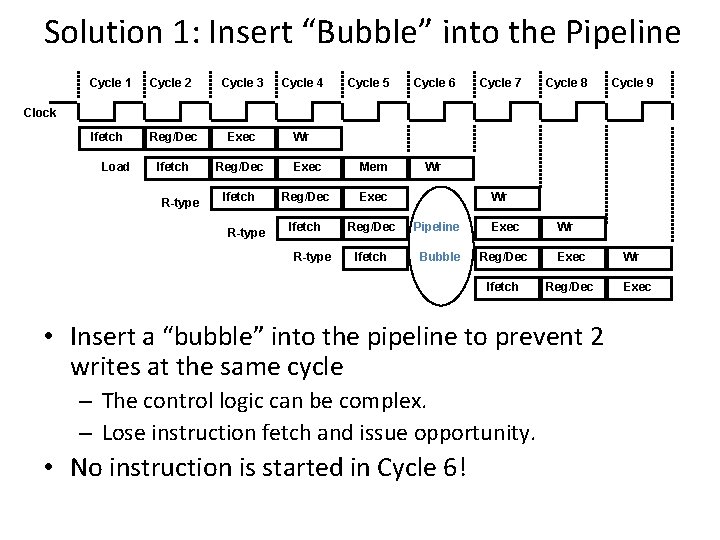
Solution 1: Insert “Bubble” into the Pipeline Cycle 1 Cycle 2 Cycle 3 Cycle 4 Cycle 5 Cycle 6 Cycle 7 Cycle 8 Ifetch Reg/Dec Exec Wr Ifetch Reg/Dec Exec Mem Ifetch Reg/Dec Exec Ifetch Reg/Dec Pipeline Exec Ifetch Bubble Reg/Dec Exec Ifetch Reg/Dec Cycle 9 Clock Load R-type Wr Wr Wr • Insert a “bubble” into the pipeline to prevent 2 writes at the same cycle – The control logic can be complex. – Lose instruction fetch and issue opportunity. • No instruction is started in Cycle 6! Wr Exec

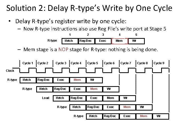
Solution 2: Delay R-type’s Write by One Cycle • Delay R-type’s register write by one cycle: – Now R-type instructions also use Reg File’s write port at Stage 5 1 R-type 3 4 Exec Mem 2 Ifetch Reg/Dec 5 Wr – Mem stage is a NOP stage for R-type: nothing is being done. Cycle 1 Cycle 2 Cycle 3 Cycle 4 Cycle 5 Cycle 6 Cycle 7 Cycle 8 Ifetch Reg/Dec Exec Mem Wr R-type Ifetch Reg/Dec Exec Mem Wr Ifetch Reg/Dec Exec Mem Cycle 9 Clock R-type Load R-type Wr

Can Pipelining Get Us Into Trouble? • Yes: Pipeline Hazards – structural hazards: attempt to use the same resource by two different instructions at the same time – data hazards: attempt to use data before it is ready • instruction source operands are produced by a prior instruction still in the pipeline • load instruction followed immediately by an ALU instruction that uses the load operand as a source value – control hazards: attempt to make a decision before condition has been evaluated • branch instructions • Can always resolve hazards by waiting – pipeline control must detect the hazard – take action (or delay action) to resolve hazards

Structural Hazard • Attempt to use same hardware for two different things at the same time. • Solution 1: Wait – Must detect hazard – Must have mechanism to stall • Solution 2: Throw more hardware at the problem

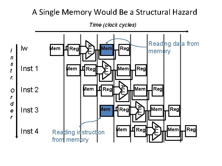
A Single Memory Would Be a Structural Hazard Time (clock cycles) Inst 4 Mem Reg Reg Mem Reg ALU Inst 3 Reg ALU Inst 2 Mem Reg ALU Inst 1 Reading data from memory Mem ALU O r d e r lw Reg ALU I n s t r. Mem Mem Reading instruction from memory Mem Reg

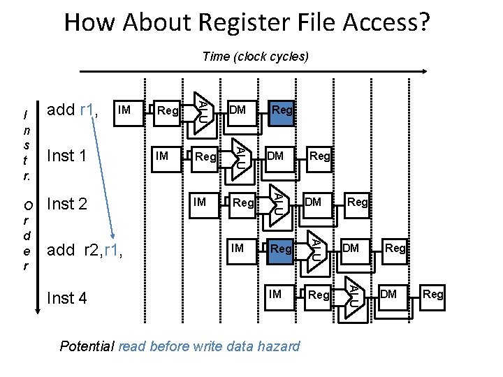
How About Register File Access? Time (clock cycles) add r 2, r 1, Inst 4 IM Reg DM IM Reg ALU Inst 2 DM ALU Inst 1 Reg ALU IM ALU O r d e r add r 1, ALU I n s t r. Reg Potential read before write data hazard Reg Reg DM Reg

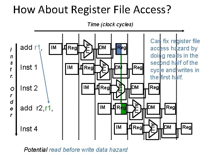
How About Register File Access? Time (clock cycles) add r 2, r 1, Inst 4 IM Reg DM IM Reg ALU Inst 2 DM ALU Inst 1 Reg ALU IM ALU O r d e r add r 1, ALU I n s t r. Can fix register file access hazard by doing reads in the second half of the cycle and writes in the first half. Reg Potential read before write data hazard Reg Reg DM Reg

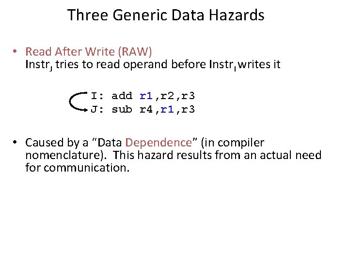
Three Generic Data Hazards • Read After Write (RAW) Instr. J tries to read operand before Instr. I writes it I: add r 1, r 2, r 3 J: sub r 4, r 1, r 3 • Caused by a “Data Dependence” (in compiler nomenclature). This hazard results from an actual need for communication.

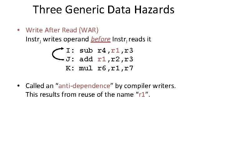
Three Generic Data Hazards • Write After Read (WAR) Instr. J writes operand before Instr. I reads it I: sub r 4, r 1, r 3 J: add r 1, r 2, r 3 K: mul r 6, r 1, r 7 • Called an “anti-dependence” by compiler writers. This results from reuse of the name “r 1”.

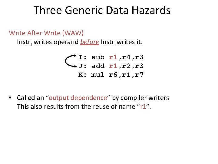
Three Generic Data Hazards Write After Write (WAW) Instr. J writes operand before Instr. I writes it. I: sub r 1, r 4, r 3 J: add r 1, r 2, r 3 K: mul r 6, r 1, r 7 • Called an “output dependence” by compiler writers This also results from the reuse of name “r 1”.

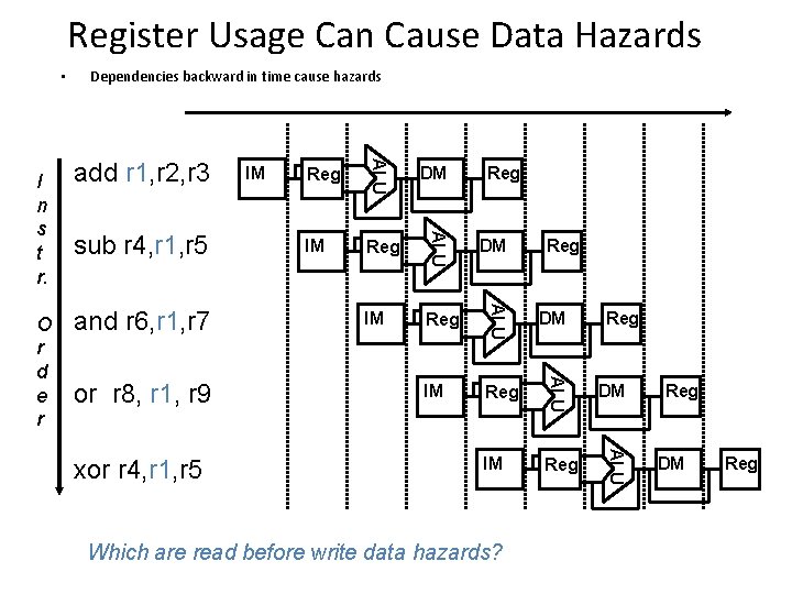
Register Usage Can Cause Data Hazards • xor r 4, r 1, r 5 IM Reg DM IM Reg ALU or r 8, r 1, r 9 DM ALU and r 6, r 1, r 7 Reg ALU sub r 4, r 1, r 5 IM ALU O r d e r add r 1, r 2, r 3 ALU I n s t r. Dependencies backward in time cause hazards Reg Which are read before write data hazards? Reg Reg DM Reg

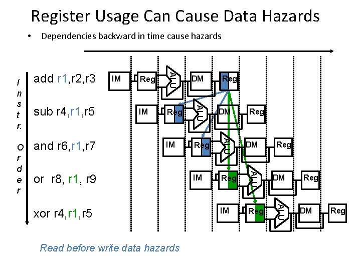
Register Usage Can Cause Data Hazards • DM IM Reg ALU and r 6, r 1, r 7 Reg ALU sub r 4, r 1, r 5 IM ALU O r d e r add r 1, r 2, r 3 ALU I n s t r. Dependencies backward in time cause hazards or r 8, r 1, r 9 xor r 4, r 1, r 5 Read before write data hazards Reg Reg DM Reg

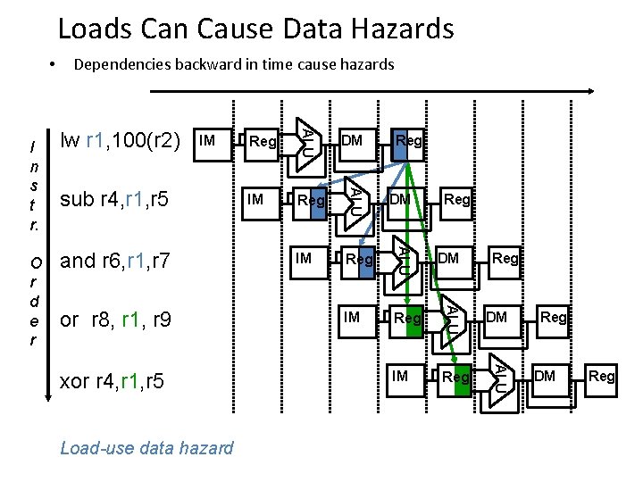
Loads Can Cause Data Hazards • or r 8, r 1, r 9 xor r 4, r 1, r 5 Load-use data hazard IM Reg DM IM Reg ALU and r 6, r 1, r 7 DM ALU sub r 4, r 1, r 5 Reg ALU IM ALU O r d e r lw r 1, 100(r 2) ALU I n s t r. Dependencies backward in time cause hazards Reg Reg DM Reg

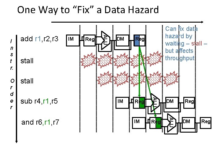
One Way to “Fix” a Data Hazard Reg DM Reg IM Reg DM IM Reg ALU IM ALU O r d e r add r 1, r 2, r 3 ALU I n s t r. Can fix data hazard by waiting – stall – but affects throughput stall sub r 4, r 1, r 5 and r 6, r 1, r 7 Reg DM Reg

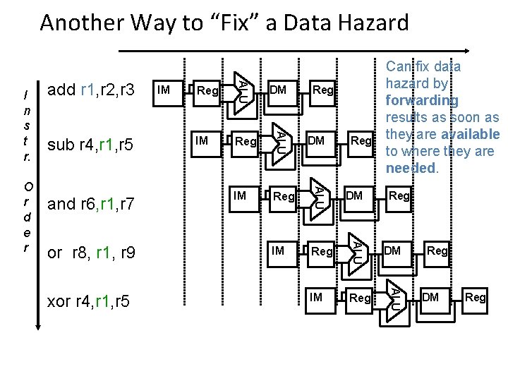
Another Way to “Fix” a Data Hazard xor r 4, r 1, r 5 IM Reg DM IM Reg ALU or r 8, r 1, r 9 DM ALU and r 6, r 1, r 7 Reg ALU sub r 4, r 1, r 5 IM ALU O r d e r add r 1, r 2, r 3 ALU I n s t r. Can fix data hazard by forwarding results as soon as they are available to where they are needed. Reg Reg DM Reg

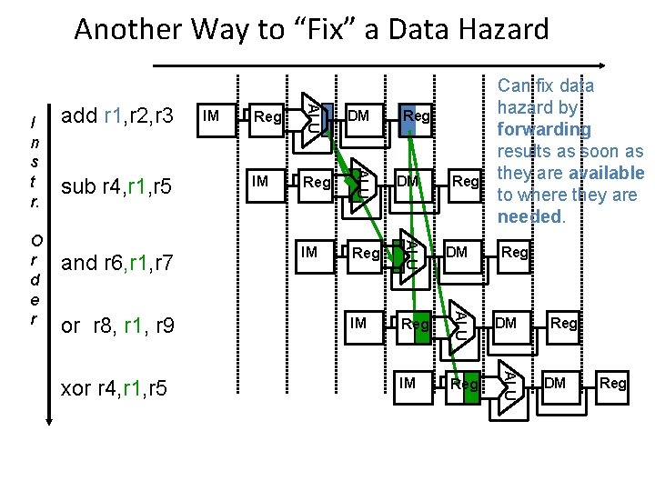
Another Way to “Fix” a Data Hazard xor r 4, r 1, r 5 IM Reg DM IM Reg ALU or r 8, r 1, r 9 DM ALU and r 6, r 1, r 7 Reg ALU sub r 4, r 1, r 5 IM ALU O r d e r add r 1, r 2, r 3 ALU I n s t r. Can fix data hazard by forwarding results as soon as they are available to where they are needed. Reg Reg DM Reg

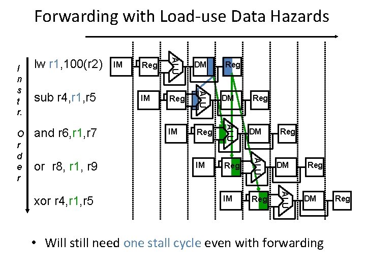
Forwarding with Load-use Data Hazards xor r 4, r 1, r 5 IM Reg DM IM Reg ALU or r 8, r 1, r 9 DM ALU and r 6, r 1, r 7 Reg ALU sub r 4, r 1, r 5 IM ALU O r d e r lw r 1, 100(r 2) ALU I n s t r. Reg Reg DM • Will still need one stall cycle even with forwarding Reg

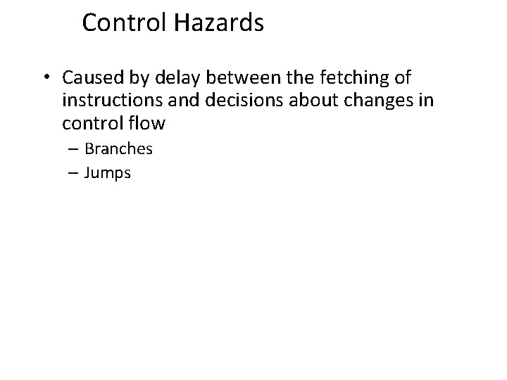
Control Hazards • Caused by delay between the fetching of instructions and decisions about changes in control flow – Branches – Jumps

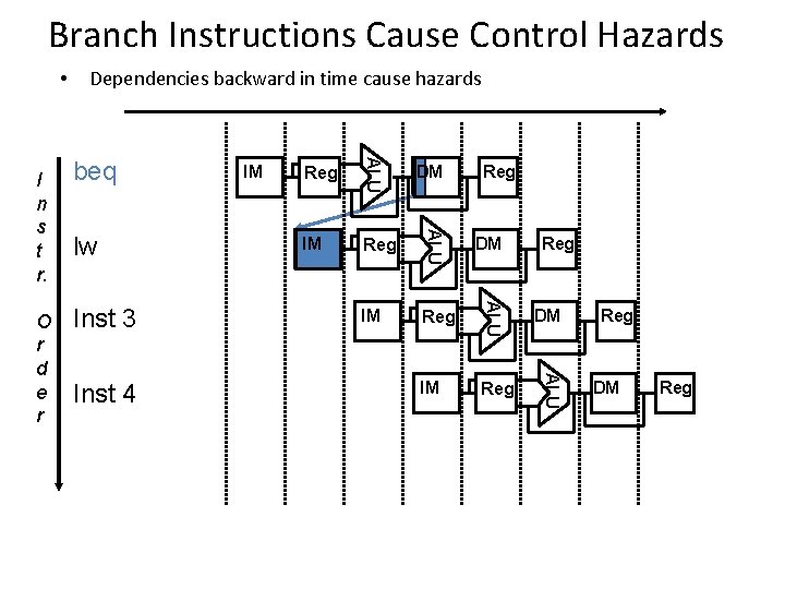
Branch Instructions Cause Control Hazards • Inst 4 IM Reg DM IM Reg ALU Inst 3 Reg ALU lw IM ALU O r d e r beq ALU I n s t r. Dependencies backward in time cause hazards DM Reg Reg DM Reg

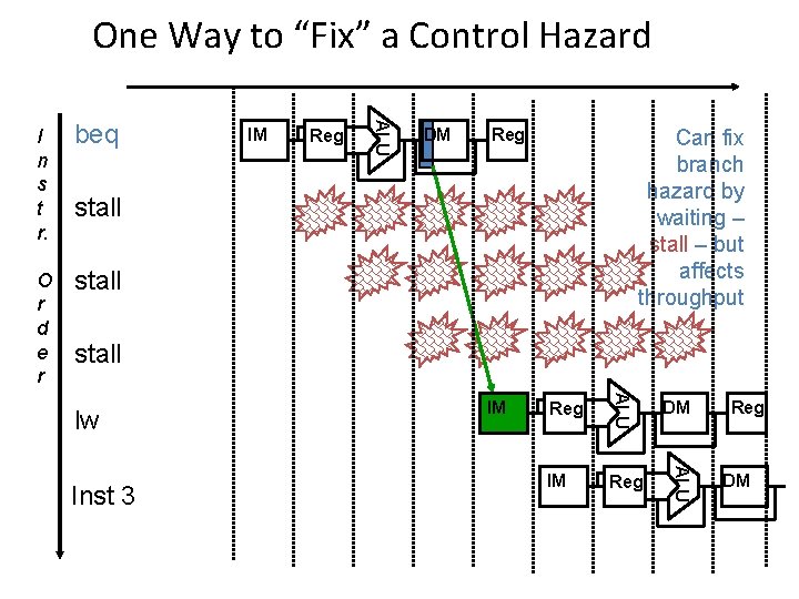
One Way to “Fix” a Control Hazard beq O r d e r stall IM Reg ALU I n s t r. DM Reg Can fix branch hazard by waiting – stall – but affects throughput stall Reg DM IM Reg ALU Inst 3 IM ALU lw Reg DM

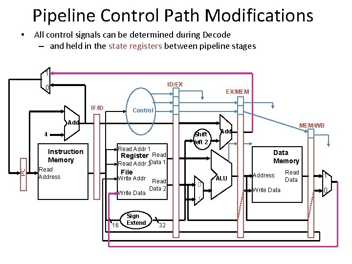
Pipeline Control Path Modifications • All control signals can be determined during Decode – and held in the state registers between pipeline stages 1 ID/EX 0 EX/MEM IF/ID Control Add Shift left 2 4 PC Instruction Memory Read Address Read Addr 1 Data Memory Register Read Addr 2 Data 1 File Write Addr Write Data 16 Sign Extend Read Data 2 0 1 32 MEM/WB Add ALU Address Write Data Read Data 1 0

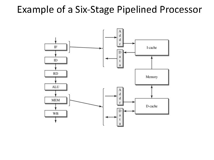
Example of a Six-Stage Pipelined Processor

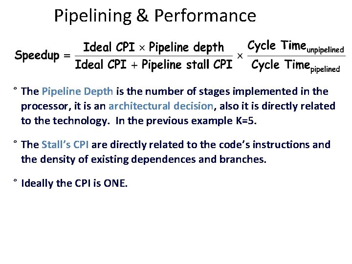
Pipelining & Performance ° The Pipeline Depth is the number of stages implemented in the processor, it is an architectural decision, also it is directly related to the technology. In the previous example K=5. ° The Stall’s CPI are directly related to the code’s instructions and the density of existing dependences and branches. ° Ideally the CPI is ONE.

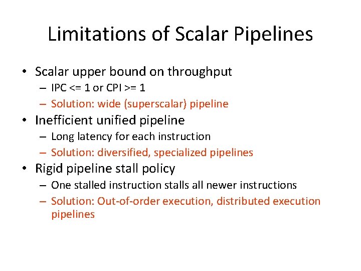
Limitations of Pipelines • Scalar upper bound on throughput – IPC <= 1 or CPI >= 1 • Inefficient unified pipeline – Long latency for each instruction • Rigid pipeline stall policy – One stalled instruction stalls all newer instructions

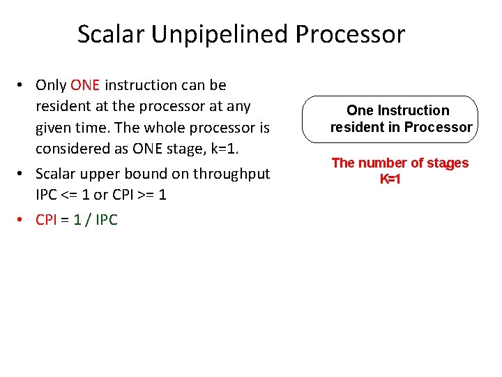
Scalar Unpipelined Processor • Only ONE instruction can be resident at the processor at any given time. The whole processor is considered as ONE stage, k=1. • Scalar upper bound on throughput IPC <= 1 or CPI >= 1 • CPI = 1 / IPC One Instruction resident in Processor The number of stages , K=1

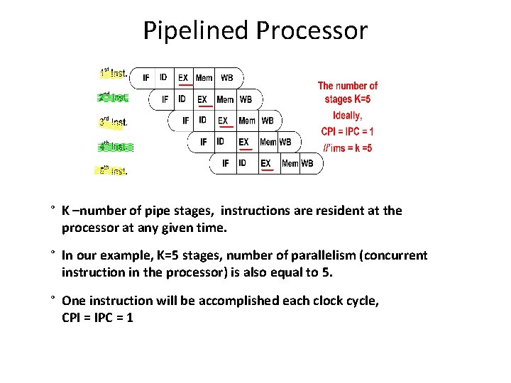
Pipelined Processor ° K –number of pipe stages, instructions are resident at the processor at any given time. ° In our example, K=5 stages, number of parallelism (concurrent instruction in the processor) is also equal to 5. ° One instruction will be accomplished each clock cycle, CPI = IPC = 1

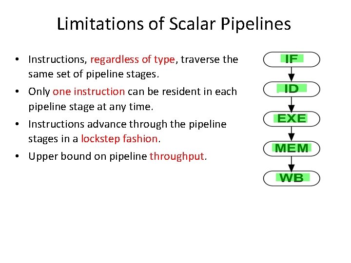
Limitations of Scalar Pipelines • Instructions, regardless of type, traverse the same set of pipeline stages. • Only one instruction can be resident in each pipeline stage at any time. • Instructions advance through the pipeline stages in a lockstep fashion. • Upper bound on pipeline throughput.

Deeper Pipeline, a Solution? • Performance is proportional to (1) Instruction Count, (2) Clock Rate, & (3) IPC –Instructions Per Clock. • Deeper pipeline has fewer logic gate levels in each stage, this leads to a shorter cycle time & higher clock rate. • But deeper pipeline can potentially incur higher penalties for dealing with inter-instruction dependences.

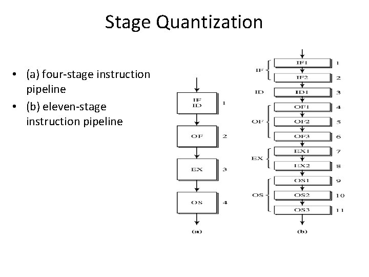
Stage Quantization • (a) four-stage instruction pipeline • (b) eleven-stage instruction pipeline

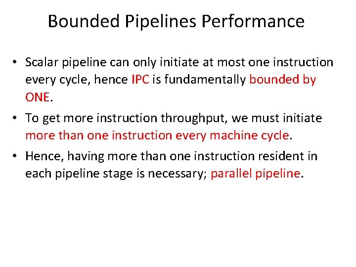
Bounded Pipelines Performance • Scalar pipeline can only initiate at most one instruction every cycle, hence IPC is fundamentally bounded by ONE. • To get more instruction throughput, we must initiate more than one instruction every machine cycle. • Hence, having more than one instruction resident in each pipeline stage is necessary; parallel pipeline.

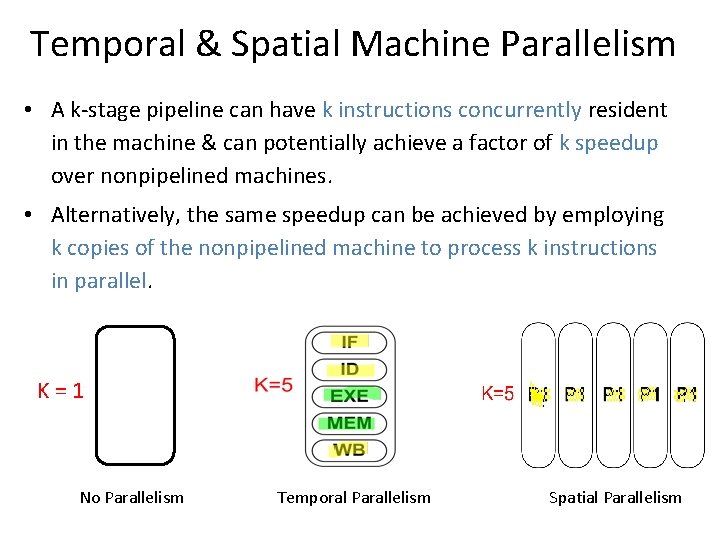
Temporal & Spatial Machine Parallelism • A k-stage pipeline can have k instructions concurrently resident in the machine & can potentially achieve a factor of k speedup over nonpipelined machines. • Alternatively, the same speedup can be achieved by employing k copies of the nonpipelined machine to process k instructions in parallel. K=1 No Parallelism Temporal Parallelism Spatial Parallelism

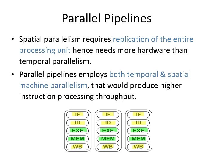
Parallel Pipelines • Spatial parallelism requires replication of the entire processing unit hence needs more hardware than temporal parallelism. • Parallel pipelines employs both temporal & spatial machine parallelism, that would produce higher instruction processing throughput.

Parallel Pipelines • For parallel pipelines, the speedup is primarily determined by the width of the parallel pipeline. • A parallel pipeline with width s can concurrently process up to s instructions in each of its pipeline stages; and produce a potential speedup of s.

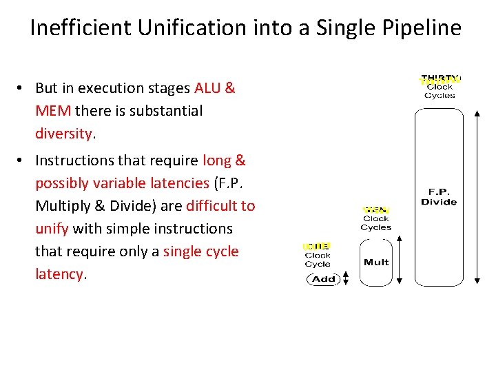
Inefficient Unification into a Single Pipeline • But in execution stages ALU & MEM there is substantial diversity. • Instructions that require long & possibly variable latencies (F. P. Multiply & Divide) are difficult to unify with simple instructions that require only a single cycle latency.

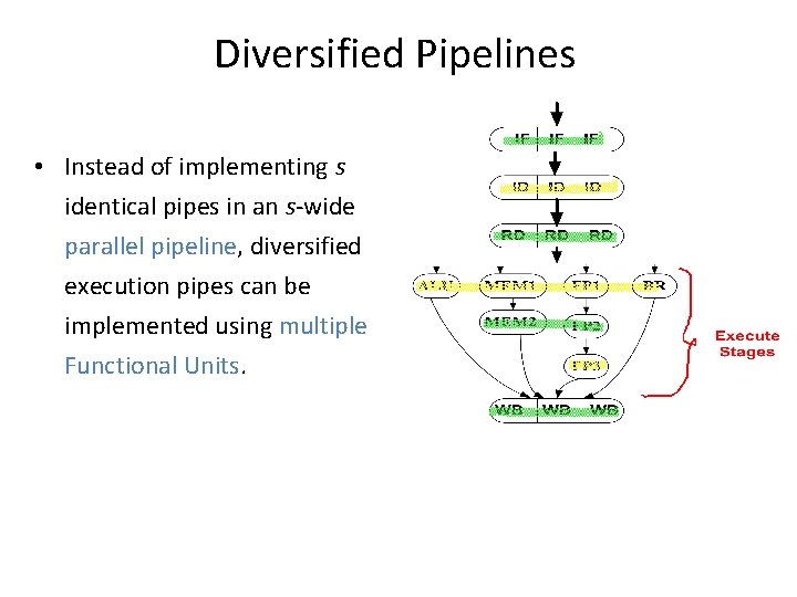
Diversified Pipelines • Specialized execution units customized for specific instruction types will contribute to the need for greater diversity in the execution stages. • For parallel pipelines, there is a strong motivation to implement multiple different execution units – subpipelines, in the execution portion of parallel pipeline. We call such pipelines diversified pipelines.

Diversified Pipelines • In a unified pipeline, though each instruction type only requires a subset of the execution stages, it must traverse all the execution stages –even if idling. • The execution latency for all instruction types is equal to the total number of execution stages; resulting in unnecessary stalling of trailing instructions.

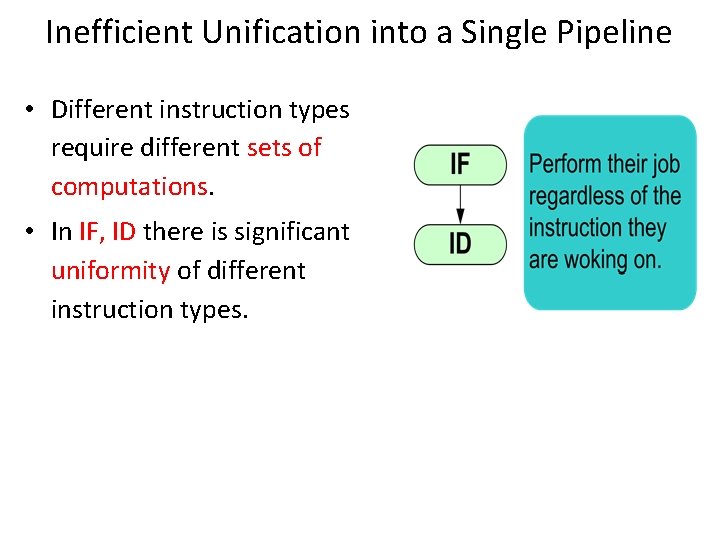
Inefficient Unification into a Single Pipeline • Different instruction types require different sets of computations. • In IF, ID there is significant uniformity of different instruction types.

Diversified Pipelines • Instead of implementing s identical pipes in an s-wide parallel pipeline, diversified execution pipes can be implemented using multiple Functional Units.

Advantages of Diversified Pipelines • Efficient hardware design due to customized pipes for particular instruction type. • Each instruction type incurs only the necessary latency & make use of all the stages. • Possible distributed & independent control of each execution pipe if all inter-instruction dependences are resolved prior to dispatching.

Diversified Pipelines Design • The number of functional units should match the available I. L. P. of the program. The mix of F. U. s should match the dynamic mix of instruction types of the program. • Most 1 st generation superscalars simply integrated a second execution pipe for processing F. P. instructions with the existing scalar pipeline.

Diversified Pipelines Design (2) • In 4 -issue machines, 4 F. U. s are implemented for executing integer, F. P. , Load/Store, & branch instructions. • Later, designs incorporated multiple integer units, some dedicated for long latency integer operations: multiply & divide, and operations for image, graphics, signal processing applications.

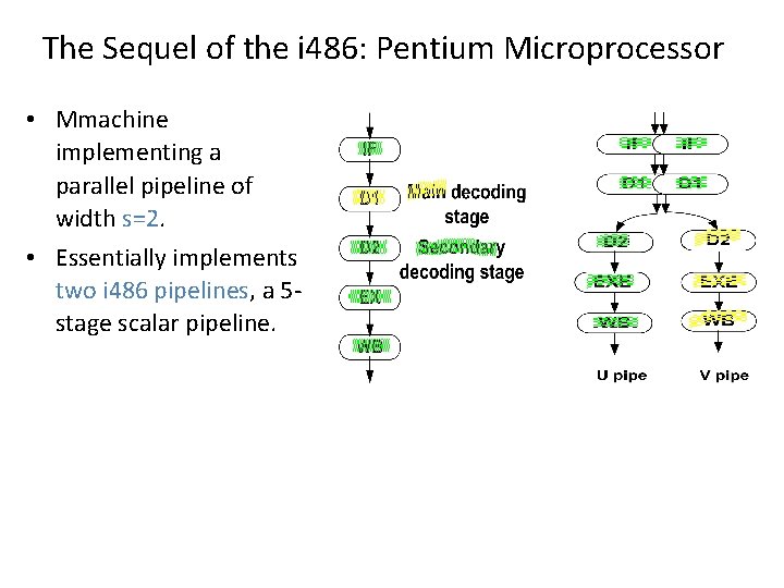
The Sequel of the i 486: Pentium Microprocessor • Mmachine implementing a parallel pipeline of width s=2. • Essentially implements two i 486 pipelines, a 5 stage scalar pipeline.

Pentium Microprocessor • Multiple instructions can be fetched & decoded by the first 2 stages of the parallel pipeline in every machine cycle. • In each cycle, potentially two instructions can be issued into the two execution pipelines. • The goal is to achieve a peak execution rate of two instructions per machine cycle. • The execute stage can perform an ALU operation or access the D-cache hence additional ports to the RF must be provided to support 2 ALU operations.

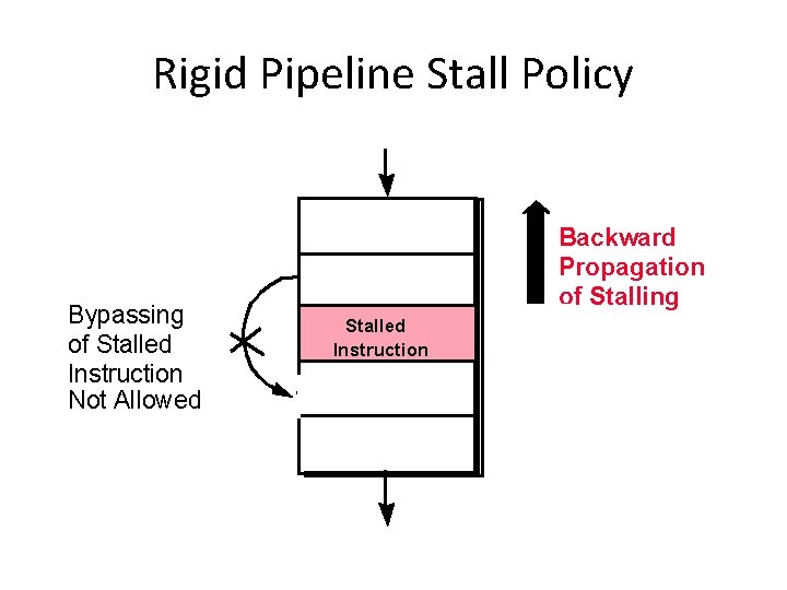
Rigid Pipeline Stall Policy Bypassing of Stalled Instruction Not Allowed Backward Propagation of Stalling Stalled Instruction

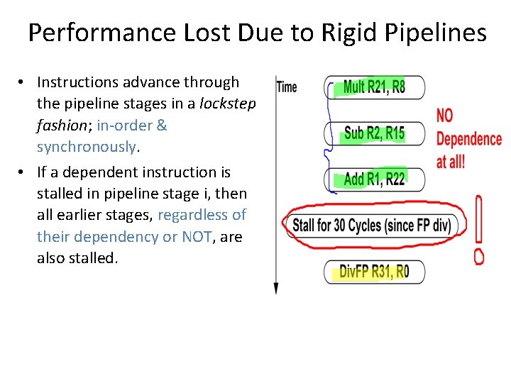
Performance Lost Due to Rigid Pipelines • Instructions advance through the pipeline stages in a lockstep fashion; in-order & synchronously. • If a dependent instruction is stalled in pipeline stage i, then all earlier stages, regardless of their dependency or NOT, are also stalled.

Rigid Pipeline Penalty • Only after the inter-instruction dependence is satisfied, that all i stalled instructions can again advance synchronously down the pipeline. • If an independent instruction is allowed to bypass the stalled instruction & continue down the pipeline stages, an idling cycle of the pipeline can be eliminated.

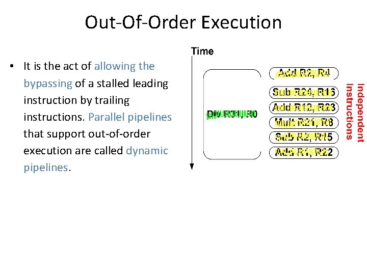
Out-Of-Order Execution • It is the act of allowing the bypassing of a stalled leading instruction by trailing instructions. Parallel pipelines that support out-of-order execution are called dynamic pipelines.

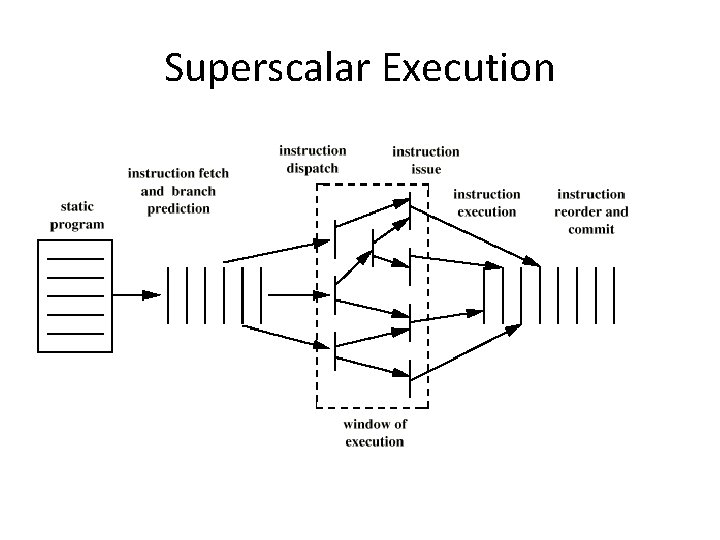
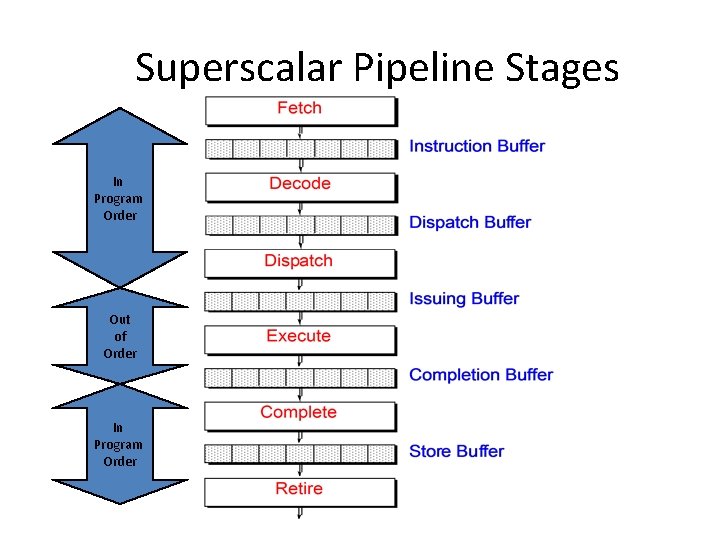
Characteristics of Superscalar Machines • Simultaneously advance multiple instructions through the pipeline stages. • Multiple functional units => higher instruction execution throughput. • Able to execute instructions in an order different from that specified by the original program. • Out of program order execution allows more parallel processing of instructions.

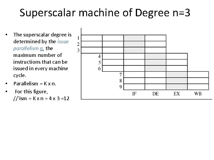
Superscalar machine of Degree n=3 • • • The superscalar degree is determined by the issue parallelism n, the maximum number of instructions that can be issued in every machine cycle. Parallelism = K x n. For this figure, //’ism = K x n = 4 x 3 =12

From Scalar to Superscalar Pipelines • Superscalar pipelines are parallel pipelines: able to initiate the processing of multiple instructions in every machine cycle. • Superscalar are diversified; they employ multiple & heterogeneous functional units in their execution stages. • They are implemented as dynamic pipelines in order to achieve the best possible performance without requiring reordering of instructions by the compiler.

Dynamic Pipelines • Superscalar pipelines differ from (rigid) scalar pipelines in one key aspect; the use of complex multi-entry buffers. • In order to minimize unnecessary staling of instructions in a parallel pipeline, trailing instructions must be allowed to bypass a stalled leading instruction. • Such bypassing can change the order of execution of instructions from the original sequential order of the static code.

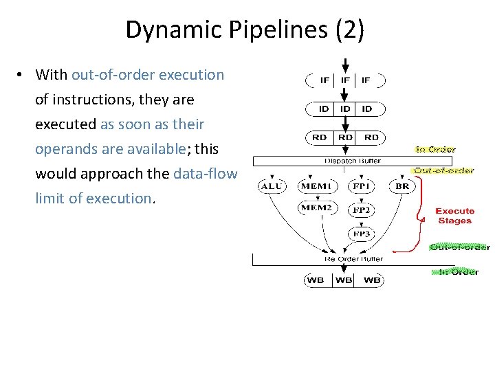
Dynamic Pipelines (2) • With out-of-order execution of instructions, they are executed as soon as their operands are available; this would approach the data-flow limit of execution.

Dynamic Pipelines (3) • A dynamic pipeline achieves out-of-order execution via the use of complex multi-entry buffers that allow instructions to enter & leave the buffers in different orders.

Superscalar Execution

Superscalar Pipeline Stages In Program Order Out of Order In Program Order

Limitations of Scalar Pipelines • Scalar upper bound on throughput – IPC <= 1 or CPI >= 1 – Solution: wide (superscalar) pipeline • Inefficient unified pipeline – Long latency for each instruction – Solution: diversified, specialized pipelines • Rigid pipeline stall policy – One stalled instruction stalls all newer instructions – Solution: Out-of-order execution, distributed execution pipelines

Extra Slides

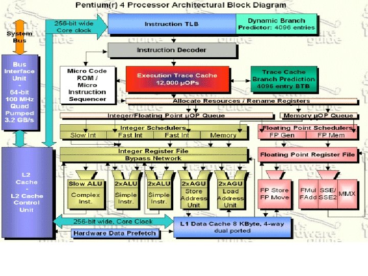
Pentium 4 • 80486 - CISC • Pentium – some superscalar components – Two separate integer execution units • Pentium Pro – Full blown superscalar • Subsequent models refine & enhance superscalar design

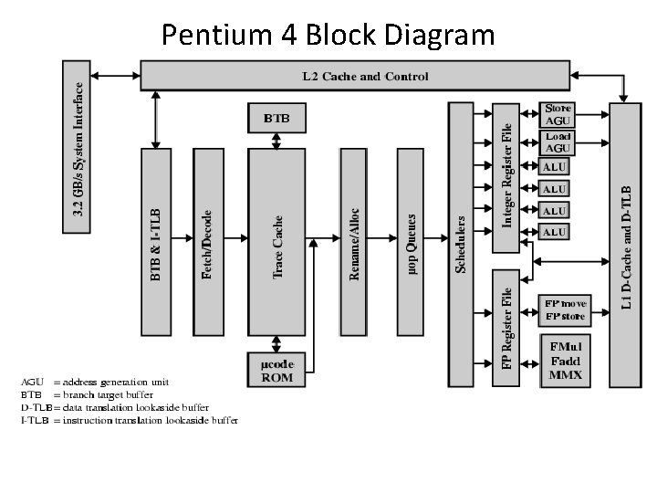
Pentium 4 Block Diagram

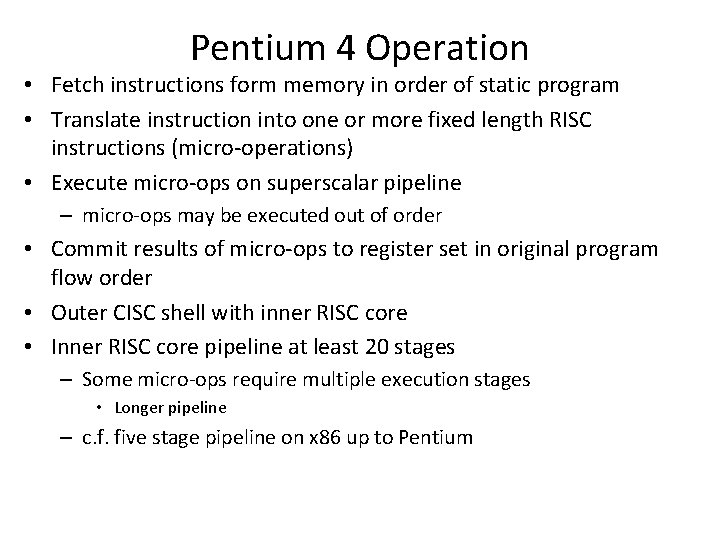
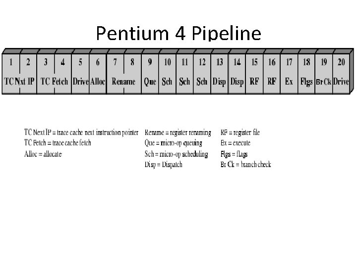
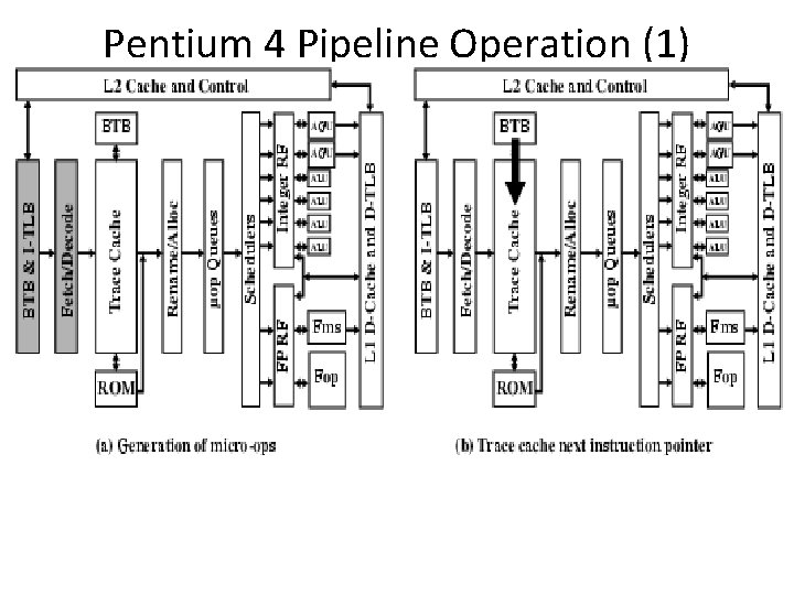
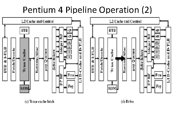
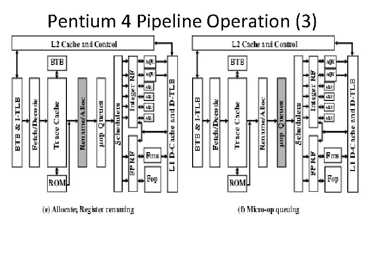
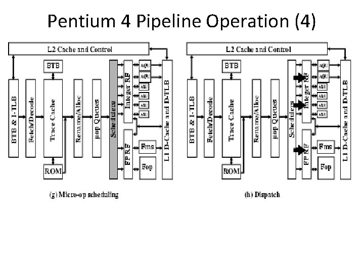
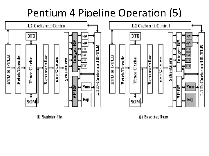
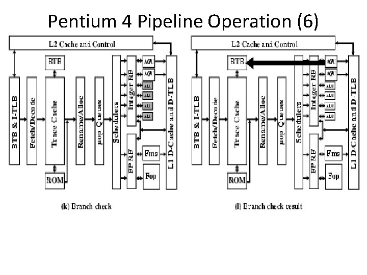
Pentium 4 Operation • Fetch instructions form memory in order of static program • Translate instruction into one or more fixed length RISC instructions (micro-operations) • Execute micro-ops on superscalar pipeline – micro-ops may be executed out of order • Commit results of micro-ops to register set in original program flow order • Outer CISC shell with inner RISC core • Inner RISC core pipeline at least 20 stages – Some micro-ops require multiple execution stages • Longer pipeline – c. f. five stage pipeline on x 86 up to Pentium

Pentium 4 Pipeline

Pentium 4 Pipeline Operation (1)

Pentium 4 Pipeline Operation (2)

Pentium 4 Pipeline Operation (3)

Pentium 4 Pipeline Operation (4)

Pentium 4 Pipeline Operation (5)

Pentium 4 Pipeline Operation (6)

Introduction to Power. PC 620 • The first 64 -bit superscalar processor to employ: – – – Aggressive branch prediction, Real out-of-order execution, Six pipelined execution units, Dynamic renaming for all register files, Distributed multientry reservation stations, A completion buffer to ensure program correctness. • Most of these features had not been previously implemented in a single-chip microprocessor.