contents Introduction Of measures of dispersion Definition of

contents � Introduction Of measures of dispersion. � Definition of Dispersion. � Range � Quartile deviation. � Mean deviation. � Standard deviation. � Variance. � Coefficient of variance. � Summary. � References.

INTRODUCTION � The Measures of central tendency gives us a birds eye view of the entire data they are called averages of the first order, �it serve to locate the centre of the distribution but they do not reveal how the items are spread out on either side of the central value. � The measure of the scattering of items in a distribution about the average is called dispersion. 5

� The measures of dispersion are also called averages of the second order because they are based on the deviations of the different values from the mean or other measures of central tendency which are called averages of the first order.

Introduction � So far we have looked at ways of summarising data by showing some sort of average (central tendency). � But it is often useful to show much these figures differ from the average. � This measure is called dispersion.

DEFINITION � In the words of Bowley “Dispersion is the measure of the variation of the items” According to Conar “Dispersion is a measure of the extent to which the individual items vary” 8

Purpose of Measuring Dispersion � A measure of dispersion appears to serve two purposes. � First, it is one of the most important quantities used to characterize a frequency distribution. � Second, it affords a basis of comparison between two or more frequency distributions. � The study of dispersion bears its importance from the fact that various distributions may have exactly the same averages, but substantial differences in their variability.

� Measures of dispersion are descriptive statistics that describe how similar a set of scores are to each other � The more similar the scores are to each other, the lower the measure of dispersion will be � The less similar the scores are to each other, the higher the measure of dispersion will be � In general, the more spread out a distribution is, the larger the measure of dispersion will be

Measures of dispersion � There are ways of showing dispersion: � Range � Inter-quartile range � Semi- interquartile range (quartile deviation) � Coefficient of quratile deviation � Mean deviation � Standard deviation � Variance � Coefficient of variation

The Range � The range is defined as the difference between the largest score in the set of data and the smallest score in the set of data, XL– XS � What is the range of the following data: 4 8 1 6 6 2 9 3 6 9 � The largest score (XL) is 9; the smallest score (XS) is 1; the range is XL- XS= 9 - 1 = 8 12

When To Use the Range � The range is used when � you have ordinal data or � you are presenting your results to people with little or no knowledge of statistics � The range is rarely used in scientific work as it is fairly insensitive � It depends on only two scores in the set of data, XL and XS � Two very different sets of data can have the same range: 1 1 9 vs 1 3 5 7 9

The Inter-Quartile Range � The inter-quartile range is the range of the middle half of the values. � It is a better measurement to use than the range because it only refers to the middle half of the results. � Basically, the extremes are omitted and cannot affect the answer.

� To calculate the inter-quartile range we must first find the quartiles. � There are three quartiles, called Q 1, Q 2 & Q 3. We do not need to worry about Q 2 (this is just the median). � Q 1 is simply the middle value of the bottom half of the data and Q 3 is the middle value of the top half of the data.

� We calculate the inter quartile range by taking Q 1 away from Q 3 (Q 3 – Q 1). Remember data must be placed in order 10 – 25 – 47 – 49 – 51 – 52 – 54 – 56 – 57 – 58 – 60 – 62 – 66 – 68 – 70 - 90 Because there is an even number of values (18) we can split them into two groups of 9. Q 1 IR = Q 3 – Q 1 , IR = 62 – 49. IR = 13 Q 3

QUARTILE DEVIATION � It is the second measure of dispersion, no doubt improved version over the range. It is based on the quartiles so while calculating this may require upper quartile (Q 3) and lower quartile (Q 1) and then is divided by 2. Hence it is half of the deference between two quartiles it is also a semi inter quartile range. The formula of Quartile Deviation is � (Q D) = Q 3 - Q 1 2 17

The Semi-Interquartile Range � The semi-interquartile range (or SIR) is defined as the difference of the first and third quartiles divided by two � The first quartile is the 25 th percentile � The third quartile is the 75 th percentile � SIR = (Q 3 - Q 1) / 2 18

COFFICIENT OF QURATILE D� EVIATION The relative measure of dispersion corrsponding to quartile deviation is known as the cofficent of quartile deviation. � QD =Q 3 -Q 1/Q 3+Q 1 � This will be always less than one and will be positive as Q 3>Q 1. � Smaller value of cofficient of QD indicates lesser variability.

Median The statistical concept of the median is a value that divides a data sample, population, or probability distribution into two halves. Finding the median essentially involves finding the value in a data sample that has a physical location between the rest of the numbers. Note that when calculating the median of a finite list of numbers, the order of the data samples is important. 2, 10, 21, 23, 38 After listing the data in ascending order, and determining that there an odd number of values, it is clear that 23 is the median given this case. If there were another value added to the data set: 2, 10, 21, 23, 38, 1027892

Mode In statistics, the mode is the value in a data set that has the highest number of recurrences. It is possible for a data set to be multimodal, meaning that it has more than one mode. For example: 2, 10, 21, 23, 38 Both 23 and 38 appear twice each, making them both a mode for the data set above.

MEAN DEVIATION �Mean Deviation is also known as average deviation. In this case deviation taken from any average especially Mean, Median or Mode. While taking deviation we have to ignore negative items and consider all of them as positive. The formula is given below 20

MEAN DEVIATION The formula of MD is given below MD = d N (deviation taken from mean) MD = m N (deviation taken from median) MD = z N (deviation taken from mode) 21

STANDARD DEVIATION � The standard deviation is represented by the Greek letter (sigma). It is always calculated from the arithmetic mean, median and mode is not considered. While looking at the earlier measures of dispersion all of them suffer from one or the other demerit i. e. � Range –it suffer from a serious drawback considers only 2 values and neglects all the other values of the series. 23

STANDARD DEVIATION � Quartile deviation considers only 50% of the item and ignores the other 50% of items in the series. � Mean deviation no doubt an improved measure but ignores negative signs without any basis. � Karl Pearson after observing all these things has given us a more scientific formula for calculating or measuring dispersion. While calculating SD we take deviations of individual observations from their AM and then each squares. The sum of the squares is divided by the number of observations. The square root of this sum is knows as standard deviation. 24

Standard Deviation � The standard deviation is one of the most important measures of dispersion. It is much more accurate than the range or inter quartile range. � It takes into account all values and is not unduly affected by extreme values.

What does it measure? � It measures the dispersion (or spread) of figures around the mean. � A large number for the standard deviation means there is a wide spread of values around the mean, whereas a small number for the standard deviation implies that the values are grouped close together around the mean.

Variance is defined as the average of the square deviations or square of standared deviation of set of observation n Sample variance: S 2 Where 2 (X X) i i 1 X = mean n = sample size Xi = ith value of the variable X n -1

The formula σ = √{∑ (x - ẍ)2 / n} This is the symbol for the standard deviation

Standard Deviation � Standard deviation is the positive square root of the mean-square deviations of the observations from their arithmetic mean. Population 2 x i N Sample s SD variance 2 x x i N 1

Standard Deviation for Group Data � SD is : s fi xi x 2 Where N s fx N i i � Simplified formula 2 f x x f fx N 2 i

Population vs. Sample. Standard. Deviation (Grouped Data)

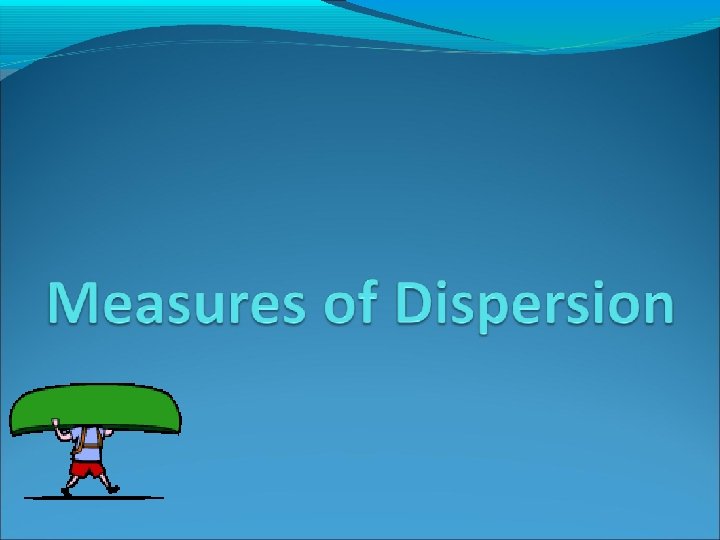
�We are going to try and find the standard deviation of the minimum temperatures of 10 weather stations in Britain on a winters day. The temperatures are: 5, 9, 3, 2, 7, 9, 8, 2, 2, 3 (˚Centigrade)

To calculate the standard deviation we construct a table like this one: x ẍ (x - ẍ)2 There should be enough space here to fit in the number of values. Eg: there are 10 temperatures so leave 10 lines. ∑x = ẍ = ∑x/n = ∑(x - ẍ)2/n = √∑(x - ẍ)2/n = x = temperature --- ẍ = mean temperature --- √ = square root ∑ = total of --- 2 = squared --- n = number of values

Next we write the values (temperatures) in To calculate the standard deviation we construct a table like th is column x (they can be in any order). one: x ẍ (x - ẍ)2 5 9 3 2 7 9 8 2 2 3 ∑x = ẍ = ∑x/n = ∑(x - ẍ)2/n = √∑(x - ẍ)2/n = x = temperature --- ẍ = mean temperature --- √ = square root ∑ = total of --- 2 = squared --- n = number of values

Add them up (∑x) x ẍ Calculate the mean (ẍ) (x - ẍ)2 5 9 3 2 7 9 8 2 2 3 ∑x = 50 ẍ = ∑x/n = 50/10 = 5 ∑(x - ẍ)2 = ∑(x - ẍ)2/n = √∑(x - ẍ)2/n = x = temperature --- ẍ = mean temperature --- √ = square root ∑ = total of --- 2 = squared --- n = number of values

Write the mean temperature (ẍ) in every row in the second column. x ẍ 5 9 3 2 7 9 8 2 2 3 5 5 5 5 5 ∑x = 50 ẍ = ∑x/n = 50/10 = 5 (x - ẍ)2 ∑(x - ẍ)2 = ∑(x - ẍ)2/n = √∑(x - ẍ)2/n = x = temperature --- ẍ = mean temperature --- √ = square root ∑ = total of --- 2 = squared --- n = number of values

Subtract each value (temperature) from the mean. It does not matter if you obtain a negative number. x ẍ (x - ẍ) 5 9 3 2 7 9 8 2 2 3 5 5 5 5 5 0 4 -2 -3 2 4 3 -3 -3 -2 ∑x = 50 ẍ = ∑x/n = 50/10 = 5 (x - ẍ)2 ∑(x - ẍ)2 = ∑(x - ẍ)2/n = √∑(x - ẍ)2/n = x = temperature --- ẍ = mean temperature --- √ = square root ∑ = total of --- 2 = squared --- n = number of values

Square (2) all of the figures you obtained in column 3 to get rid of the negative numbers. x ẍ (x - ẍ)2 5 9 3 2 7 9 8 2 2 3 5 5 5 5 5 0 4 -2 -3 2 4 3 -3 -3 -2 0 16 4 9 4 16 9 9 9 4 ∑x = 50 ẍ = ∑x/n = 50/10 = 5 ∑(x - ẍ)2 = ∑(x - ẍ)2/n = √∑(x - ẍ)2/n = x = temperature --- ẍ = mean temperature --- √ = square root ∑ = total of --- 2 = squared --- n = number of values

Add up all of the figures that you calculated in column 4 to get ∑ (x - ẍ)2. x ẍ (x - ẍ)2 5 9 3 2 7 9 8 2 2 3 5 5 5 5 5 0 4 -2 -3 2 4 3 -3 -3 -2 0 16 4 9 4 16 9 9 9 4 ∑x = 50 ẍ = ∑x/n = 50/10 = 5 ∑(x - ẍ)2 = 80 ∑(x - ẍ)2/n = √∑(x - ẍ)2/n = x = temperature --- ẍ = mean temperature --- √ = square root ∑ = total of --- 2 = squared --- n = number of values

Divide ∑(x - ẍ)2 by the total number of values (in this case 10 – weather stations) x ẍ (x - ẍ)2 5 9 3 2 7 9 8 2 2 3 5 5 5 5 5 0 4 -2 -3 2 4 3 -3 -3 -2 0 16 4 9 4 16 9 9 9 4 ∑x = 50 ẍ = ∑x/n = 50/10 = 5 ∑(x - ẍ)2 = 80 ∑(x - ẍ)2/n = 8 √∑(x - ẍ)2/n = x = temperature --- ẍ = mean temperature --- √ = square root ∑ = total of --- 2 = squared --- n = number of values

Take the square root (√) of the figure to obtain the standard deviation. (Round your answer to the nearest decimal place) x ẍ (x - ẍ)2 5 9 3 2 7 9 8 2 2 3 5 5 5 5 5 0 4 -2 -3 2 4 3 -3 -3 -2 0 16 4 9 4 16 9 9 9 4 ∑x = 50 ẍ = ∑x/n = 50/10 = 5 ∑(x - ẍ)2 = 80 ∑(x - ẍ)2/n = 8 √∑(x - ẍ)2/n = x = temperature --- ẍ = mean temperature --- √ = square root ∑ = total of --- 2 = squared --- n = number of values

2. 8°C

Why? � Standard deviation is much more useful. � For example our 2. 8 means that there is a 68% chance of the temperature falling within ± 2. 8°C of the mean temperature of 5°C. � That is one standard deviation away from the mean. Normally, values are said to lie between one, two or three standard deviations from the mean.

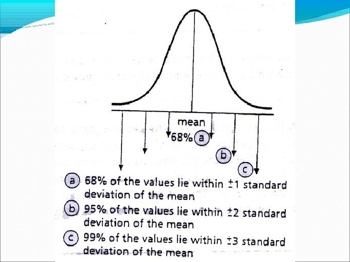
Where did the 68% come from? This is a normal distribution curve. It is a bell-shaped curve with most of the data cluster around the mean value and where the data gradually declines the further you get from the mean until very few data appears at the extremes.

Most people are near average height. Some are short But few are very short Some are tall And few are very tall.

If you look at the graph you can see that most of the data (68%) is located within 1 standard deviation on either side of the mean, even more (95%) is located within 2 standard deviations on either side of the mean, and almost all (99%) of the data is located within 3 standard deviations on either side of the mean.

Example-1: Find Standard Deviation of Ungroup Data Family No. 1 2 3 4 5 6 7 8 9 10 Size (xi) 3 3 4 4 5 5 6 6 7 7

x Here, Family No. xi xi x 2 xi x n i 50 10 5 1 2 3 4 5 6 7 8 9 10 Total 3 3 4 4 5 5 6 6 7 7 50 -2 4 -2 -1 -1 0 0 1 1 2 2 0 4 1 1 0 0 1 1 4 4 20 9 9 16 16 25 25 36 36 49 49 270 2 s 2 x i x 2 n 1 20 2. 2, 9 s 2. 2 1. 48

Example-2: Find Standard Deviation of Group Data xi x 2 x i x 2 f i x i x 2 fi f i xi 3 2 6 18 -3 9 18 5 3 15 75 -1 1 3 7 2 14 98 1 1 2 8 2 16 128 2 4 8 9 1 9 81 3 9 9 Total 10 60 400 - - 40 xi x f i i i 60 6 10 s 2 f i xi f x i x 2 i n 1 40 4. 44 9

What Does the Variance Formula Mean? � Variance is the mean of the squared deviation scores � The larger the variance is, the more the scores deviate, on average, away from the mean � The smaller the variance is, the less the scores deviate, on average, from the mean 52

(This will seem easy compared to the standard deviation!)

Coefficient of variation � The coefficient of variation indicates the spread of values around the mean by a percentage. Coefficient of variation = Standard Deviation x 100 mean

Things you need to know � The higher the Coefficient of Variation the more widely spread the values are around the mean. � The purpose of the Coefficient of Variation is to let us compare the spread of values between different data sets.

Coefficient of Variation Measures relative variation Always in percentage (%) Shows variation relative to mean Can be used to compare two or more sets of data measured in different units S 100% CV X

Comparing Coefficient of Variation Stock A: Average price last year = $50 Standard deviation = $5 S $5 CVA 100% 10% $50 X Stock B: Average price last year = $100 Standard deviation = $5 S $5 100% 5% CVB $100 X Both stocks have the same standard deviation, but stock B is less variable relative to its price

Sample vs. Population CV

Calculate! Calculate the coefficient of variation for the following data set. The price, in cents, of a stock over five trading days was 52, 58, 55, 57, 59.

Solution

Example-: Comments on Children in a community Height weight Mean 40 inch 10 kg SD CV 5 inch 0. 125 2 kg 0. 20 � Since the coefficient of variation for weight is greater than that of height, we would tend to conclude that weight has more variability than height in the population.