Measures of Dispersion or Measures of Variability Measures

Measures of Dispersion or Measures of Variability

Measures of Variability § A single summary figure that describes the spread of observations within a distribution.

MEASURES OF DESPERSION § § RANGE INTERQUARTILE RANGE VARIANCE STANDARD DEVIATION

Measures of Variability § Range § Difference between the smallest and largest observations. § Interquartile Range § Range of the middle half of scores. § Variance § Mean of all squared deviations from the mean. § Standard Deviation § Measure of the average amount by which observations deviate from the mean. The square root of the variance.

Variability Example: Range § Las Vegas Hotel Rates 52, 76, 100, 136, 186, 196, 205, 150, 257, 264, 280, 282, 283, 303, 317, 325, 373, 384, 400, 402, 417, 422, 472, 480, 643, 693, 732, 749, 750, 791, 891 § Range: 891 -52 = 839

Pros and Cons of the Range § Pros § Very easy to compute. § Scores exist in the data set. § Cons § Value depends only on two scores. § Very sensitive to outliers. § Influenced by sample size (the larger the sample, the larger the range).

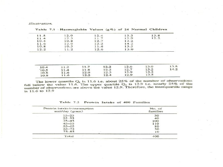
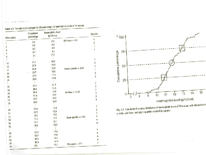
Inter quartile Range § The inter quartile range is Q 3 -Q 1 § 50% of the observations in the distribution are in the inter quartile range. § The following figure shows the interaction between the quartiles, the median and the inter quartile range.

Inter quartile Range

Quartiles: Inter quartile : IQR = Q 3 – Q 1

Pros and Cons of the Interquartile Range § Pros § Fairly easy to compute. § Scores exist in the data set. § Eliminates influence of extreme scores. § Cons § Discards much of the data.

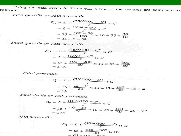
Percentiles and Quartiles § Maximum is 100 th percentile: 100% of values lie at or below the maximum § Median is 50 th percentile: 50% of values lie at or below the median § Any percentile can be calculated. But the most common are 25 th (1 st Quartile) and 75 th (3 rd Quartile)

Locating Percentiles in a Frequency Distribution § A percentile is a score below which a specific percentage of the distribution falls. § The 75 th percentile is a score below which 75% of the cases fall. § The median is the 50 th percentile: 50% of the cases fall below it § Another type of percentile : The lower quartile is 25 th percentile and the upper quartile is the 75 th percentile

Locating Percentiles in a Frequency Distribution 25 th percentile 50 th percentile 80 th percentile 25% included here 50% included here 80% included here

Five Number Summary § § § Minimum Value 1 st Quartile Median 3 rd Quartile Maximum Value

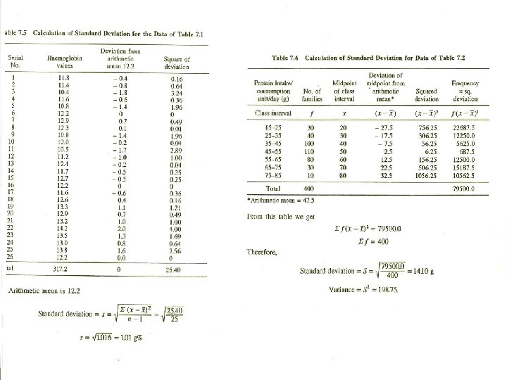
VARIANCE: Deviations of each observation from the mean, then averaging the sum of squares of these deviations. STANDARD DEVIATION: “ ROOT- MEANS-SQUARE-DEVIATIONS”

Variance § The average amount that a score deviates from the typical score. § Score – Mean = Difference Score § Average of Difference Scores = 0 § In order to make this number not 0, square the difference scores ( negatives to become positives).

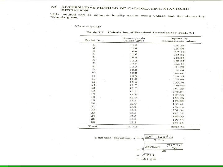
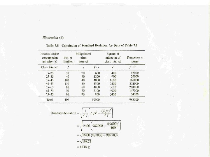
Variance: Computational Formula § Population § Sample

Variance § Use the computational formula to calculate the variance.

Variability Example: Variance § Las Vegas Hotel Rates

Pros and Cons of Variance § Pros § Takes all data into account. § Lends itself to computation of other stable measures (and is a prerequisite for many of them). § Cons § Hard to interpret. § Can be influenced by extreme scores.

Standard Deviation § To “undo” the squaring of difference scores, take the square root of the variance. § Return to original units rather than squared units.

Quantifying Uncertainty § Standard deviation: measures the variation of a variable in the sample. § Technically,

Standard Deviation Measure of the average amount by which observations deviate on either side of the mean. The square root of the variance. § Population § Sample

Variability Example: Standard Deviation Mean: 6 Standard Deviation: 2

Variability Example: Standard Deviation Mean: $371. 60 Standard Deviation:

Pros and Cons of Standard Deviation § Pros § Lends itself to computation of other stable measures (and is a prerequisite for many of them). § Average of deviations around the mean. § Majority of data within one standard deviation above or below the mean. § Cons § Influenced by extreme scores.

Mean and Standard Deviation § Using the mean and standard deviation together: § Is an efficient way to describe a distribution with just two numbers. § Allows a direct comparison between distributions that are on different scales.

A 100 samples were selected. Each of the sample contained 100 normal individuals. The mean Systolic BP of each sample is presented 110, 140, 110, 120, 130, 160, 100, 130, etc Systolic BP level 90 100 110 120 130 140 150 160 - 90, 120, 100, 120, No. of samples 5 10 20 34 20 10 5 2 Mean = 120 Sd. , = 10

Normal Distribution Mean = 120 SD = 10 90 100 110 120 130 140 150 • The curve describes probability of getting any range of values ie. , P(x>120), P(x<100), P(110 <X<130) • Area under the curve = probability • Area under the whole curve =1 • Probability of getting specific number =0, eg P(X=120) =0
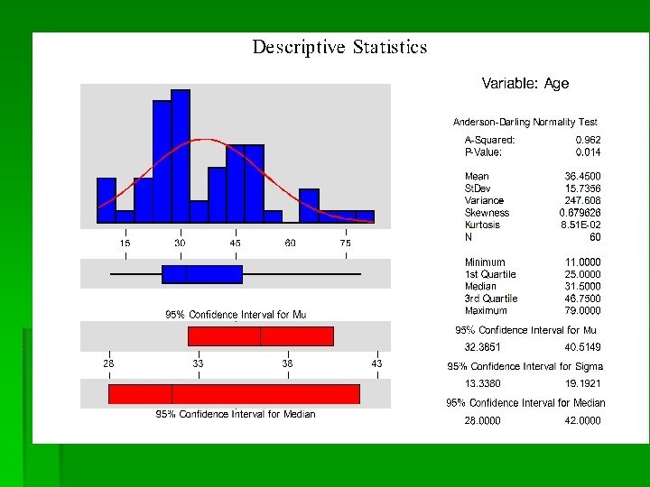

WHICH MEASURE TO USE ? DISTRIBUTION OF DATA IS SYMMETRIC ---- USE MEAN & S. D. , DISTRIBUTION OF DATA IS SKEWED ---- USE MEDIAN & QUARTILES

ANY QUESTIONS

THANK YOU
- Slides: 40