Atmospheric Dispersion General considerations on atmospheric dispersion Lagrangian

Atmospheric Dispersion • • • General considerations on atmospheric dispersion Lagrangian representation of turbulence Eulerian representation of turbulence Lagrangian models of atmospheric dispersion Eulerian models of atmospheric dispersion Street-canyon models

Atmospheric Dispersion is due to atmospheric turbulence because molecular diffusion is too slow at the time scales relevant to air pollution Molecular diffusion coefficient: ~10 -5 m 2/s Turbulent diffusion coefficient: ~1 m 2/s (stable) to ~100 m 2/s (unstable)

Lagrangian and Eulerian Representations The lagrangian representation of atmospheric dispersion follows the motion of the pollutants (particles or molecules) with respect to the mean motion of the air parcel (e. g. , the stack plume). The eulerian representation followsthe motion of the pollutants with respect to a fixed reference system (for example a surface monitoring station).

Lagrangian Representation One assumes that the dispersion process is stochastic (random) and that the atmospheric conditions are uniform and stationary: this leads to a gaussian distribution of the pollutant around the plume centerline. The concentration integrated over a crosswind plane multiplied by the wind speed must be equal to the emission rate: mass conservation of the emitted pollutant. If a gaussian distribution is assumed, then the volume of the puff that is within one standard deviation (s) from the puff center corresponds to 68 % of the initial mass emitted, within 2 s, 95 %, and within 3 s, 99. 7 %.

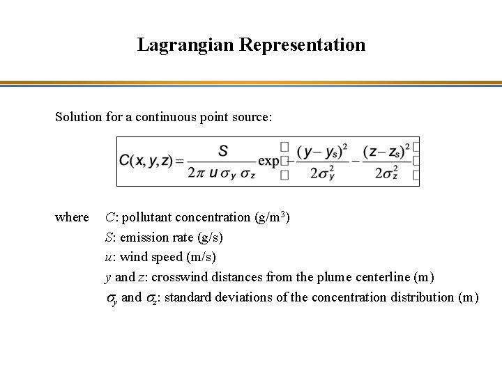
Lagrangian Representation Solution for a continuous point source: where C: pollutant concentration (g/m 3) S: emission rate (g/s) u: wind speed (m/s) y and z: crosswind distances from the plume centerline (m) sy and sz: standard deviations of the concentration distribution (m)

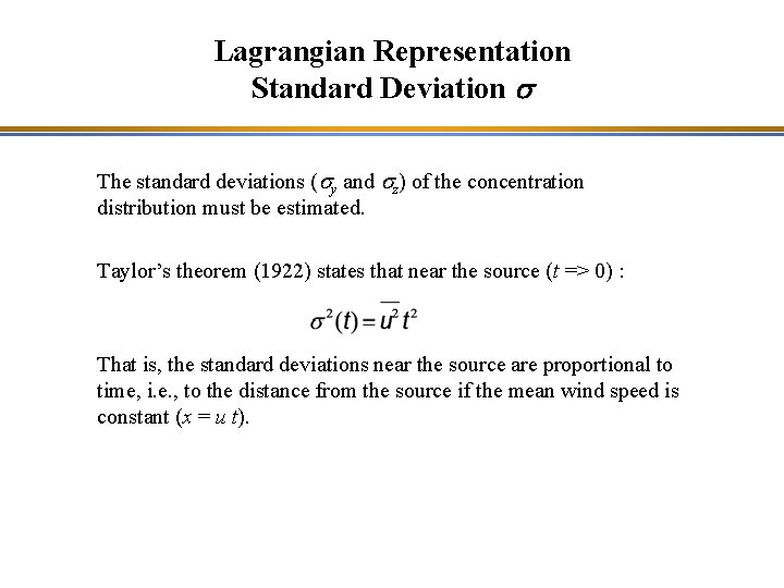
Lagrangian Representation Standard Deviation s The standard deviations (sy and sz) of the concentration distribution must be estimated. Taylor’s theorem (1922) states that near the source (t => 0) : That is, the standard deviations near the source are proportional to time, i. e. , to the distance from the source if the mean wind speed is constant (x = u t).

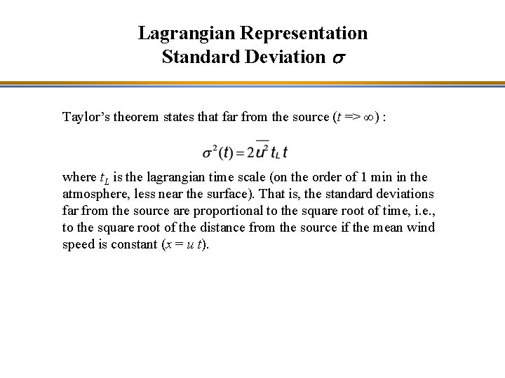
Lagrangian Representation Standard Deviation s Taylor’s theorem states that far from the source (t => ∞) : where t. L is the lagrangian time scale (on the order of 1 min in the atmosphere, less near the surface). That is, the standard deviations far from the source are proportional to the square root of time, i. e. , to the square root of the distance from the source if the mean wind speed is constant (x = u t).

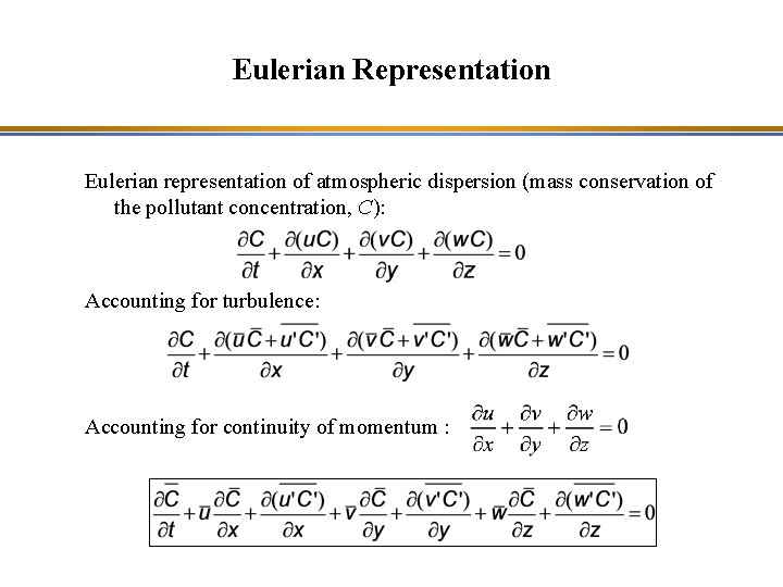
Eulerian Representation Eulerian representation of atmospheric dispersion (mass conservation of the pollutant concentration, C): Accounting for turbulence: Accounting for continuity of momentum :

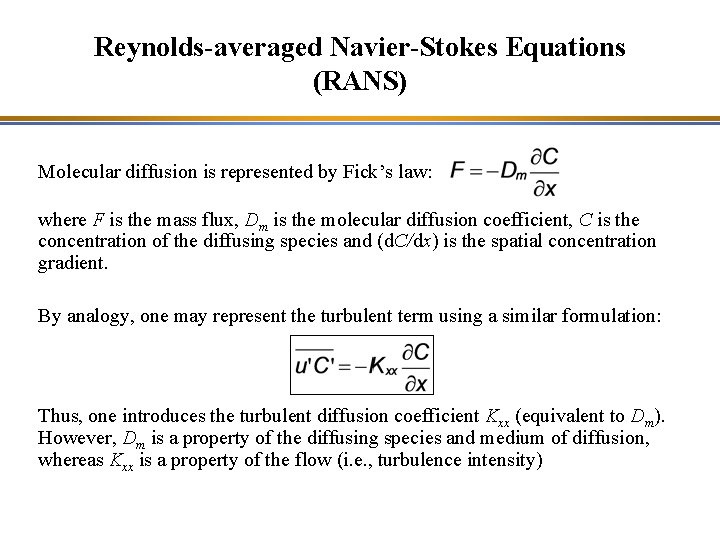
Reynolds-averaged Navier-Stokes Equations (RANS) Molecular diffusion is represented by Fick’s law: where F is the mass flux, Dm is the molecular diffusion coefficient, C is the concentration of the diffusing species and (d. C/dx) is the spatial concentration gradient. By analogy, one may represent the turbulent term using a similar formulation: Thus, one introduces the turbulent diffusion coefficient Kxx (equivalent to Dm). However, Dm is a property of the diffusing species and medium of diffusion, whereas Kxx is a property of the flow (i. e. , turbulence intensity)

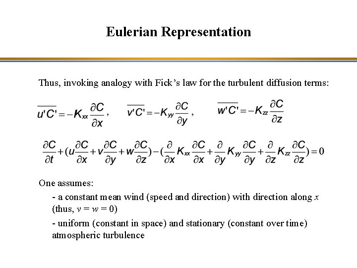
Eulerian Representation Thus, invoking analogy with Fick’s law for the turbulent diffusion terms: , , One assumes: - a constant mean wind (speed and direction) with direction along x (thus, v = w = 0) - uniform (constant in space) and stationary (constant over time) atmospheric turbulence

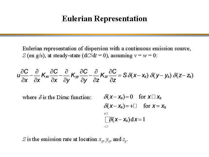
Eulerian Representation Eulerian representation of dispersion with a continuous emission source, S (en g/s), at steady-state (d. C/dt = 0), assuming v = w = 0: where d is the Dirac function: S is the emission rate at location xs, ys, and zs.

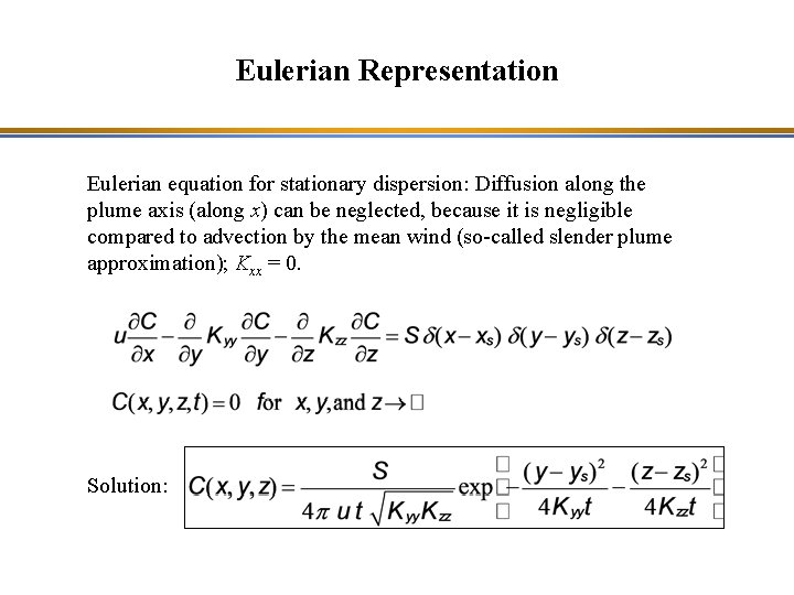
Eulerian Representation Eulerian equation for stationary dispersion: Diffusion along the plume axis (along x) can be neglected, because it is negligible compared to advection by the mean wind (so-called slender plume approximation); Kxx = 0. Solution:

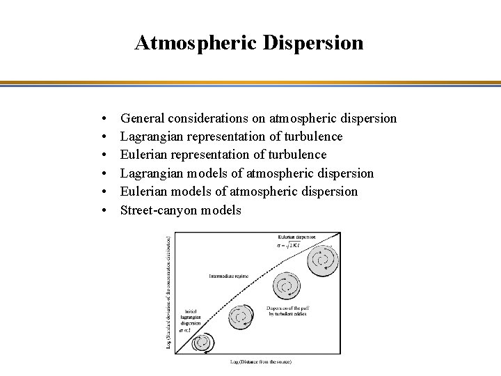
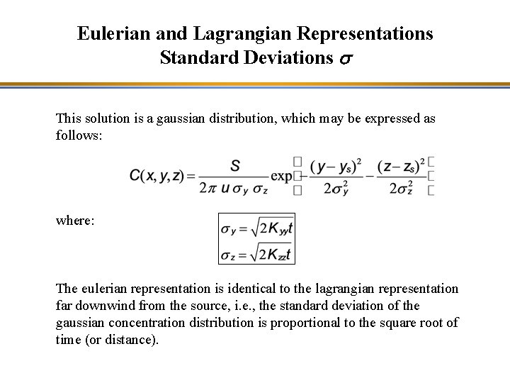
Eulerian and Lagrangian Representations Standard Deviations s This solution is a gaussian distribution, which may be expressed as follows: where: The eulerian representation is identical to the lagrangian representation far downwind from the source, i. e. , the standard deviation of the gaussian concentration distribution is proportional to the square root of time (or distance).

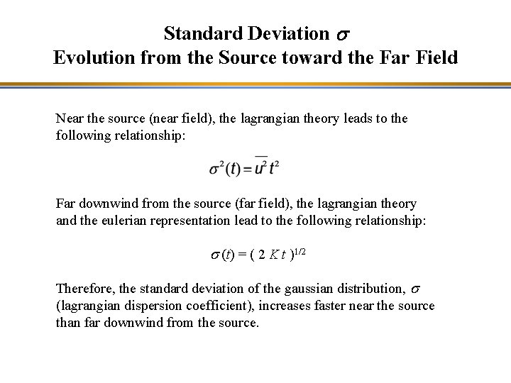
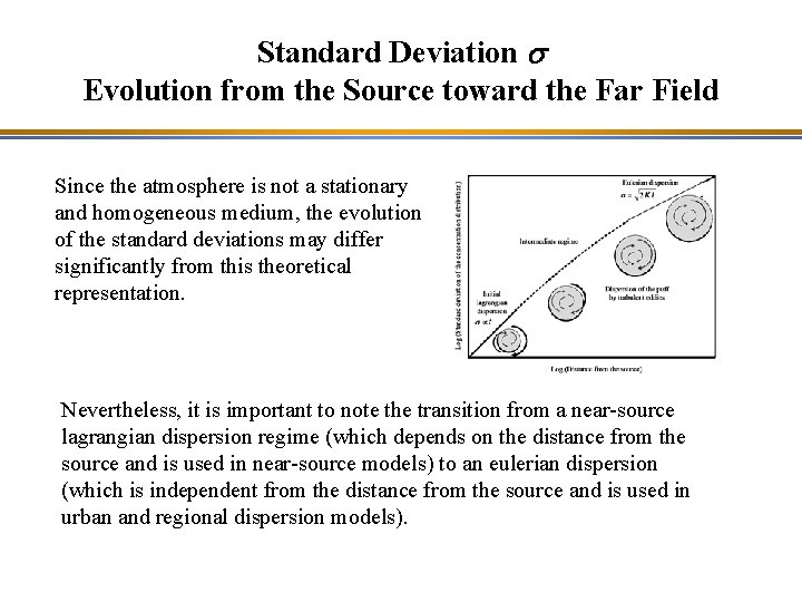
Standard Deviation s Evolution from the Source toward the Far Field Near the source (near field), the lagrangian theory leads to the following relationship: Far downwind from the source (far field), the lagrangian theory and the eulerian representation lead to the following relationship: s (t) = ( 2 K t )1/2 Therefore, the standard deviation of the gaussian distribution, s (lagrangian dispersion coefficient), increases faster near the source than far downwind from the source.

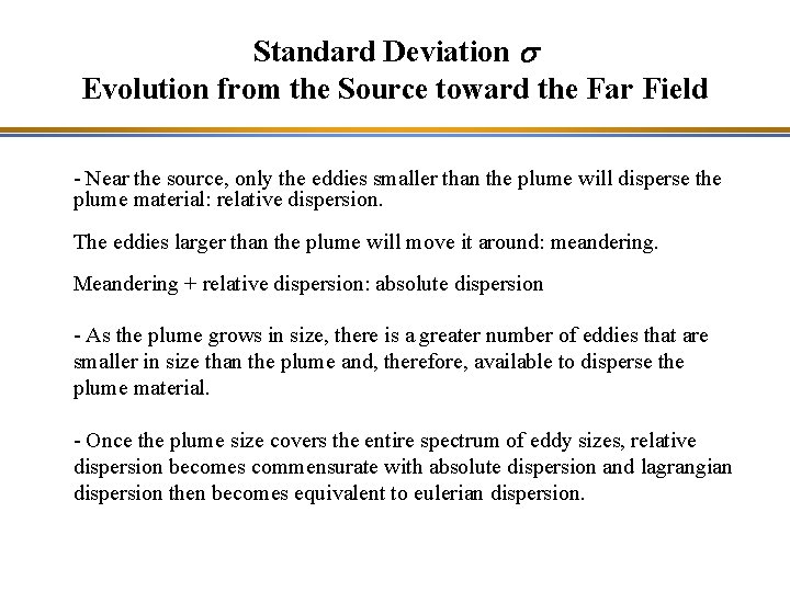
Standard Deviation s Evolution from the Source toward the Far Field - Near the source, only the eddies smaller than the plume will disperse the plume material: relative dispersion. The eddies larger than the plume will move it around: meandering. Meandering + relative dispersion: absolute dispersion - As the plume grows in size, there is a greater number of eddies that are smaller in size than the plume and, therefore, available to disperse the plume material. - Once the plume size covers the entire spectrum of eddy sizes, relative dispersion becomes commensurate with absolute dispersion and lagrangian dispersion then becomes equivalent to eulerian dispersion.

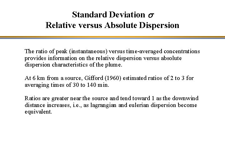
Standard Deviation s Relative versus Absolute Dispersion The ratio of peak (instantaneous) versus time-averaged concentrations provides information on the relative dispersion versus absolute dispersion characteristics of the plume. At 6 km from a source, Gifford (1960) estimated ratios of 2 to 3 for averaging times of 30 to 140 min. Ratios are greater near the source and tend toward 1 as the downwind distance increases, i. e. , as lagrangian and eulerian dispersion become equivalent.

Standard Deviation s Evolution from the Source toward the Far Field

Standard Deviation s Evolution from the Source toward the Far Field Since the atmosphere is not a stationary and homogeneous medium, the evolution of the standard deviations may differ significantly from this theoretical representation. Nevertheless, it is important to note the transition from a near-source lagrangian dispersion regime (which depends on the distance from the source and is used in near-source models) to an eulerian dispersion (which is independent from the distance from the source and is used in urban and regional dispersion models).

Plume Dispersion as a Function of Atmospheric Stability

Atmospheric Dispersion Models Lagrangian dispersion models (use of s dispersion coefficients) - Gaussian plume models - Gaussian puff models - Lagrangian “particle” models Eulerian dispersion models (use of K dispersion coefficients) - Chemical-transport models - Computational fluid dynamics (CFD) models Hybrid models - Combination of lagrangian models imbedded within an eulerian model

Gaussian Models Gaussian models can be used to simulate atmospheric dispersion of nonreactive air pollutants near their source of emission. The two main categories are: - Stationary plume models* - Puff models (which may be non-stationary) * Stationary: the inputs (emission, meteorology) are constant over time (generally with an hourly time step) and, for meteorology, spatially uniform.

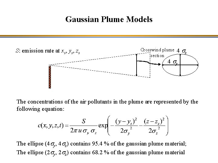
Gaussian Plume Models S: emission rate at xs, ys, zs Crosswind plume section 4 sz 4 sy The concentrations of the air pollutants in the plume are represented by the following equation: The ellipse (4 sy, 4 sz) contains 95. 4 % of the gaussian plume material; The ellipse (2 sy, 2 sz) contains 68. 2 % of the gaussian plume material

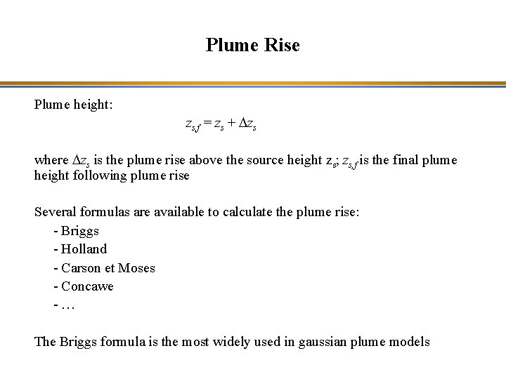
Plume Rise Plume height: zs, f = zs + Dzs where Dzs is the plume rise above the source height zs; zs, f is the final plume height following plume rise Several formulas are available to calculate the plume rise: - Briggs - Holland - Carson et Moses - Concawe -… The Briggs formula is the most widely used in gaussian plume models

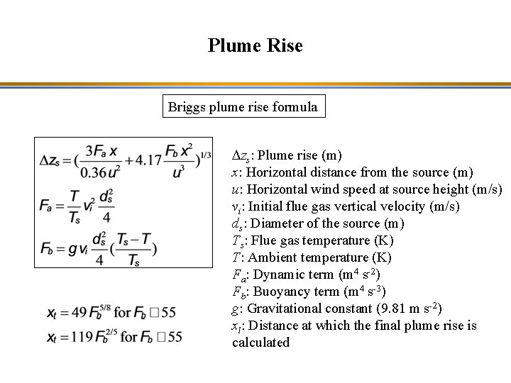
Plume Rise Briggs plume rise formula Dzs: Plume rise (m) x: Horizontal distance from the source (m) u: Horizontal wind speed at source height (m/s) vi: Initial flue gas vertical velocity (m/s) ds: Diameter of the source (m) Ts: Flue gas temperature (K) T: Ambient temperature (K) Fa: Dynamic term (m 4 s-2) Fb: Buoyancy term (m 4 s-3) g: Gravitational constant (9. 81 m s-2) xl: Distance at which the final plume rise is calculated

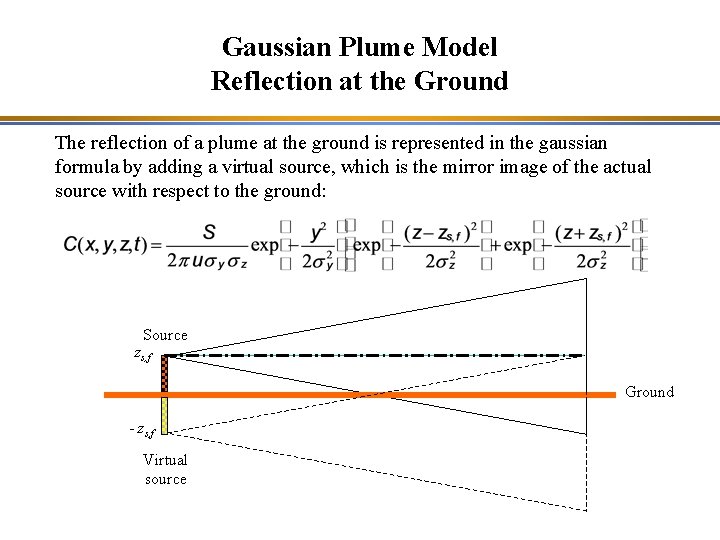
Gaussian Plume Model Reflection at the Ground The reflection of a plume at the ground is represented in the gaussian formula by adding a virtual source, which is the mirror image of the actual source with respect to the ground: Source zs, f Ground - zs, f Virtual source

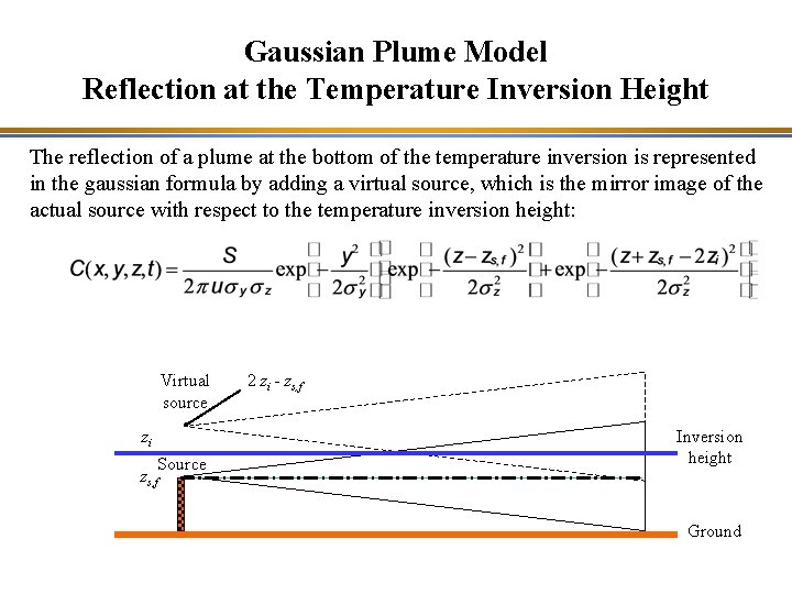
Gaussian Plume Model Reflection at the Temperature Inversion Height The reflection of a plume at the bottom of the temperature inversion is represented in the gaussian formula by adding a virtual source, which is the mirror image of the actual source with respect to the temperature inversion height: Virtual source zi Source zs, f 2 zi - zs, f Inversion height Ground

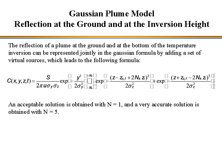
Gaussian Plume Model Reflection at the Ground at the Inversion Height The reflection of a plume at the ground at the bottom of the temperature inversion can be represented jointly in the gaussian formula by adding a set of virtual sources, which leads to the following formula: An acceptable solution is obtained with N = 1, and a very accurate solution is obtained with N = 5.

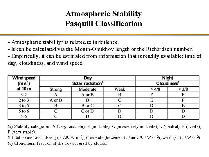
Atmospheric Stability Pasquill Classification - Atmospheric stabilitya is related to turbulence. - It can be calculated via the Monin-Obukhov length or the Richardson number. - Empirically, it can be estimated from information that is readily available: time of day, cloudiness, and wind speed. (a) Stability categories: A (very unstable), B (unstable), C (moderately unstable), D (neutral), E (stable), F (very stable). (b) Solar radiation: strong (> 700 W m-2), moderate (between 350 and 700 W m-2), weak (< 350 W m-2) (c) Cloudiness: fraction of the sky covered by clouds.

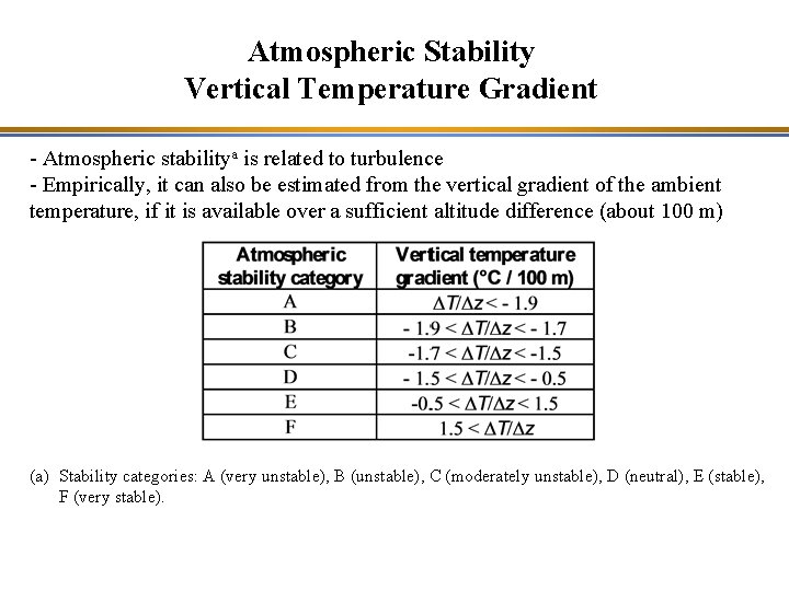
Atmospheric Stability Vertical Temperature Gradient - Atmospheric stabilitya is related to turbulence - Empirically, it can also be estimated from the vertical gradient of the ambient temperature, if it is available over a sufficient altitude difference (about 100 m) (a) Stability categories: A (very unstable), B (unstable), C (moderately unstable), D (neutral), E (stable), F (very stable).

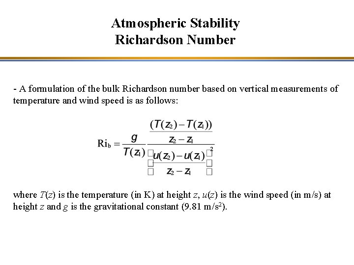
Atmospheric Stability Richardson Number - A formulation of the bulk Richardson number based on vertical measurements of temperature and wind speed is as follows: where T(z) is the temperature (in K) at height z, u(z) is the wind speed (in m/s) at height z and g is the gravitational constant (9. 81 m/s 2).

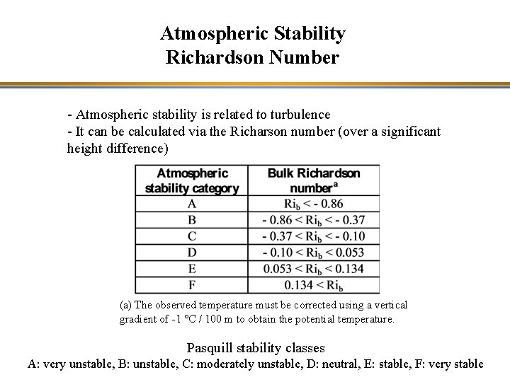
Atmospheric Stability Richardson Number - Atmospheric stability is related to turbulence - It can be calculated via the Richarson number (over a significant height difference) (a) The observed temperature must be corrected using a vertical gradient of -1 °C / 100 m to obtain the potential temperature. Pasquill stability classes A: very unstable, B: unstable, C: moderately unstable, D: neutral, E: stable, F: very stable

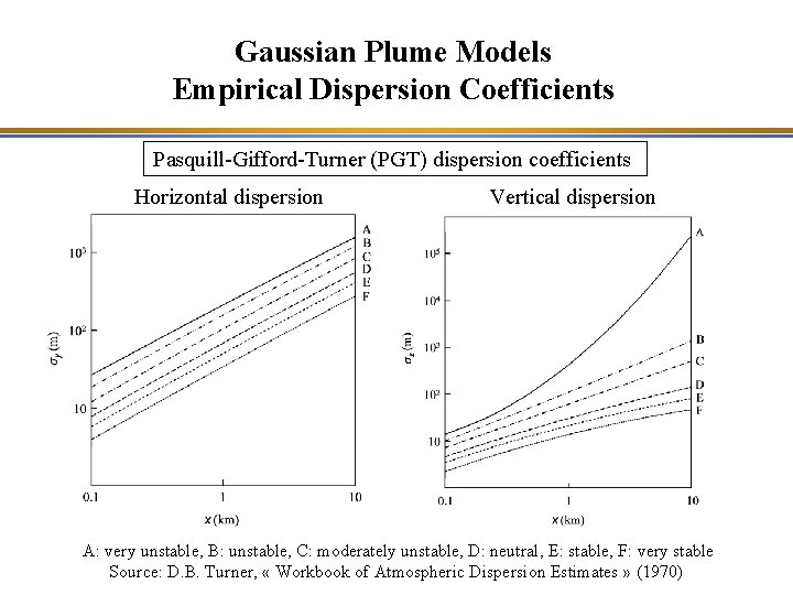
Gaussian Plume Models Empirical Dispersion Coefficients Pasquill-Gifford-Turner (PGT) dispersion coefficients Horizontal dispersion Vertical dispersion A: very unstable, B: unstable, C: moderately unstable, D: neutral, E: stable, F: very stable Source: D. B. Turner, « Workbook of Atmospheric Dispersion Estimates » (1970)

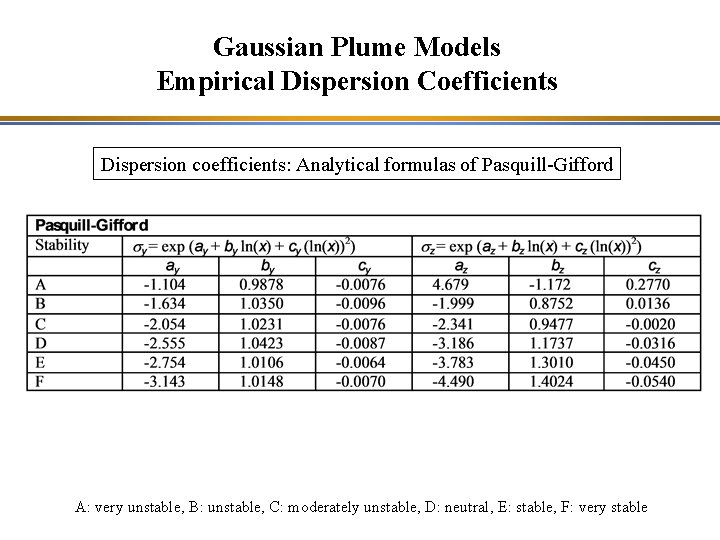
Gaussian Plume Models Empirical Dispersion Coefficients Dispersion coefficients: Analytical formulas of Pasquill-Gifford A: very unstable, B: unstable, C: moderately unstable, D: neutral, E: stable, F: very stable

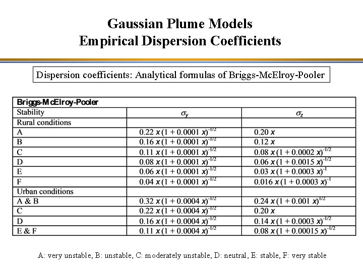
Gaussian Plume Models Empirical Dispersion Coefficients Dispersion coefficients: Analytical formulas of Briggs-Mc. Elroy-Pooler A: very unstable, B: unstable, C: moderately unstable, D: neutral, E: stable, F: very stable

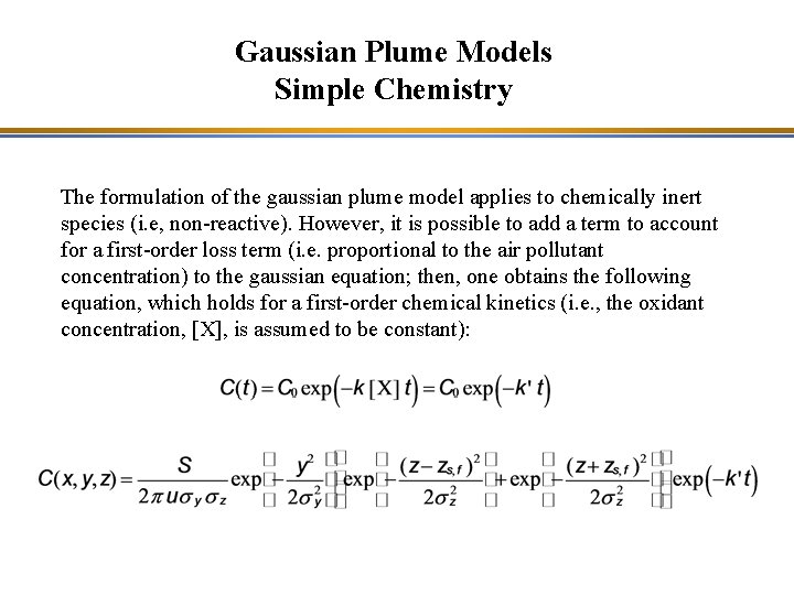
Gaussian Plume Models Simple Chemistry The formulation of the gaussian plume model applies to chemically inert species (i. e, non-reactive). However, it is possible to add a term to account for a first-order loss term (i. e. proportional to the air pollutant concentration) to the gaussian equation; then, one obtains the following equation, which holds for a first-order chemical kinetics (i. e. , the oxidant concentration, [X], is assumed to be constant):

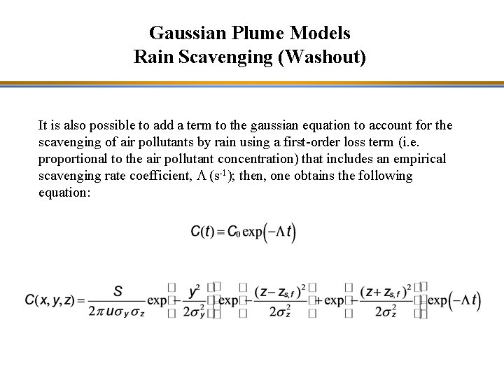
Gaussian Plume Models Rain Scavenging (Washout) It is also possible to add a term to the gaussian equation to account for the scavenging of air pollutants by rain using a first-order loss term (i. e. proportional to the air pollutant concentration) that includes an empirical scavenging rate coefficient, L (s-1); then, one obtains the following equation:

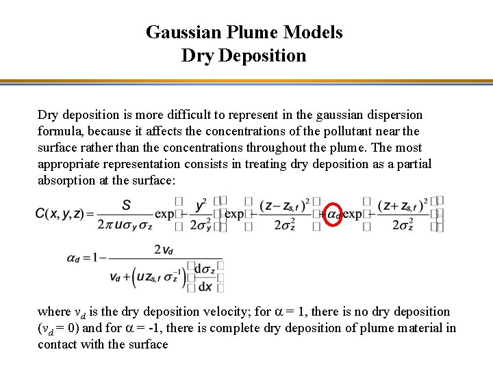
Gaussian Plume Models Dry Deposition Dry deposition is more difficult to represent in the gaussian dispersion formula, because it affects the concentrations of the pollutant near the surface rather than the concentrations throughout the plume. The most appropriate representation consists in treating dry deposition as a partial absorption at the surface: where vd is the dry deposition velocity; for a = 1, there is no dry deposition (vd = 0) and for a = -1, there is complete dry deposition of plume material in contact with the surface

Gaussian Plume Models Limitations - Gaussian models have limitations that result from the hypotheses associated with their formulation: - They do not apply far from sources (appropriate if x < 50 km). - They apply to flat terrain: approximations can be made to treat specific cases (e. g. , hill), but they cannot treat certain configurations (e. g. , streetcanyon). - They apply to simple meteorological conditions: they can take into account the effect of an elevated inversion layer, but they cannot treat wind shear for example.

Lagrangian Models - Lagrangian models, as gaussian models, calculate air pollutant concentrations with respect to a reference system that follows the trajectory of the mean wind. However, the hypothesis of stationary conditions (i. e. , constant wind speed and direction) is no longer necessary. - There are two major categories of lagrangian models: - 2 D Gridded lagrangian models with an expanding grid positioned crosswind - Lagrangian puff and “particle” models

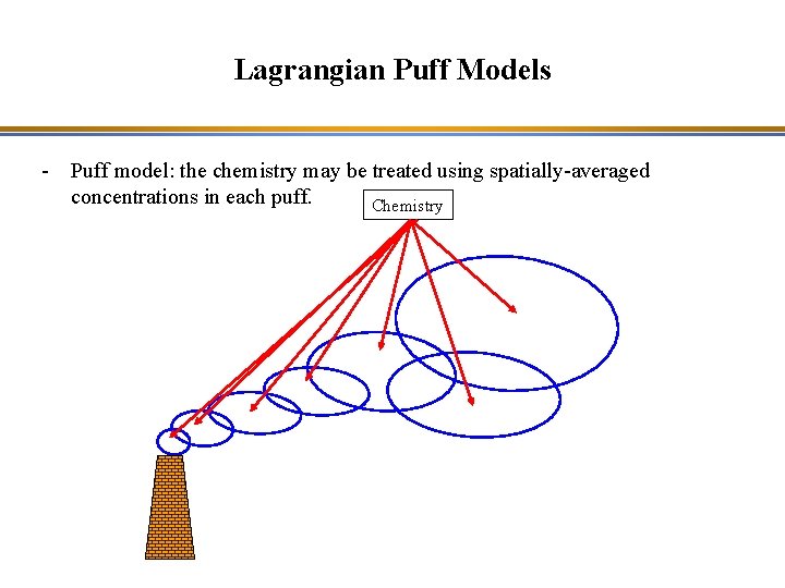
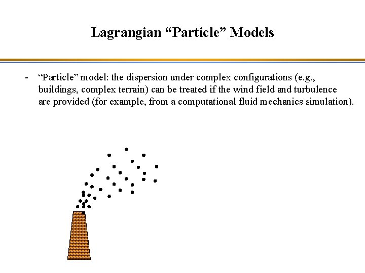
Lagrangian Puff Models - Puff and “particle” lagrangian models can handle complex wind fields, such as wind shear, because distinct puffs or “particles” can follow different trajectories. - Individual puffs may use gaussian concentration profiles; however, the puff ensemble, which constitutes the plume, does not necessarily show gaussian concentration profiles because of the different trajectories followed by the individual puffs. Some approximations must be made for the atmospheric chemistry because average concentrations are typically assumed for each individual puff. - “Particle” models cannot treat chemistry because there is no air volume associated with the “particles”.

Lagrangian Puff Models - Puff model: the chemistry may be treated using spatially-averaged concentrations in each puff. Chemistry

Lagrangian “Particle” Models - “Particle” model: the dispersion under complex configurations (e. g. , buildings, complex terrain) can be treated if the wind field and turbulence are provided (for example, from a computational fluid mechanics simulation).

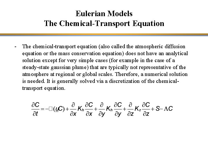
Eulerian Models The Chemical-Transport Equation - The chemical-transport equation (also called the atmospheric diffusion equation or the mass conservation equation) does not have an analytical solution except for very simple cases (for example in the case of a steady-state gaussian plume) that are typically not representative of the atmosphere at regional or global scales. Therefore, a numerical solution is needed. It is generally solved via a discretization of the chemicaltransport equation.

Eulerian Models Various Representations of Vertical Dispersion

Eulerian Models Representation of Vertical Dispersion (Kz)

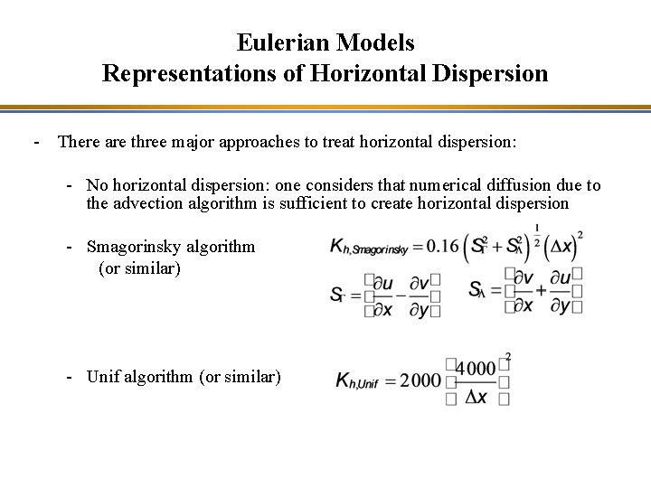
Eulerian Models Representations of Horizontal Dispersion - There are three major approaches to treat horizontal dispersion: - No horizontal dispersion: one considers that numerical diffusion due to the advection algorithm is sufficient to create horizontal dispersion - Smagorinsky algorithm (or similar) - Unif algorithm (or similar)

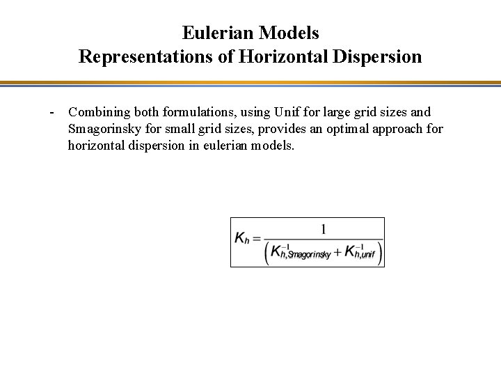
Eulerian Models Representations of Horizontal Dispersion - Smagorinsky algorithm - The dispersion coefficient is proportional to the horizontal grid surface area, X 2. - Numerical diffusion increases with the grid size. - Therefore, the Smagorinsky algorithm leads to an increase in horizontal dispersion as the grid resolution becomes coarser.

Eulerian Models Representations of Horizontal Dispersion - Unif algorithm - The dispersion coefficient is inversely proportional to the horizontal grid surface area: X-2. - Numerical diffusion increases with the grid size. - Therefore, the Unif algorithm leads to an increase in horizontal dispersion as the grid resolution becomes finer.

Eulerian Models Representations of Horizontal Dispersion - Combining both formulations, using Unif for large grid sizes and Smagorinsky for small grid sizes, provides an optimal approach for horizontal dispersion in eulerian models.

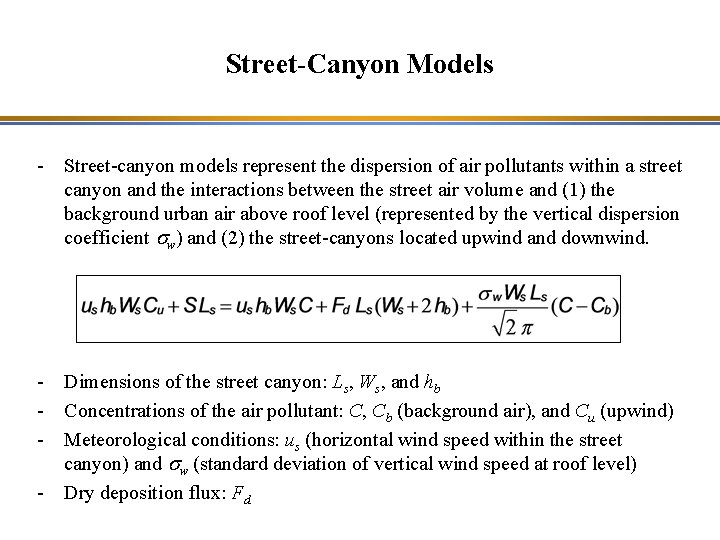
Street-Canyon Models - Street-canyon models represent the dispersion of air pollutants within a street canyon and the interactions between the street air volume and (1) the background urban air above roof level (represented by the vertical dispersion coefficient sw) and (2) the street-canyons located upwind and downwind. - Dimensions of the street canyon: Ls, Ws, and hb - Concentrations of the air pollutant: C, Cb (background air), and Cu (upwind) - Meteorological conditions: us (horizontal wind speed within the street canyon) and sw (standard deviation of vertical wind speed at roof level) - Dry deposition flux: Fd

Eulerian and Lagrangian Models Hybrid (Plume-in-grid) Models - If one wants to simulate background air pollution (urban or regional) and near -field pollution, one may construct a hybrid model, which simulates background air pollution in an eulerian grid system and the near-source air pollution with a lagrangian approach (using puffs, plumes or simple parameterizations) embedded within the eulerian model. This approach is called “plume-in-grid” (Pin. G) modeling (although it may actually use puff models to simulate the plumes) or multi-scale modeling. - Hybrid models offer several advantages: - Representation of the near-source pollution at the sub-grid level - Correct treatment of atmospheric dispersion and chemistry for the plumes emitted from large point sources (stacks of power plants, cement plants, refineries…), volume sources (fugitive emissions from refineries, chemical plants…), and line sources (major roads and freeways, airplanes, ships, street canyons…).

Computational Fluid Dynamics (CFD) Models - CFD models can provide a large array of parameterizations of turbulence with very fine spatial resolution and complex configurations: - K-theory k-e k-w Large eddy simulation (LES)

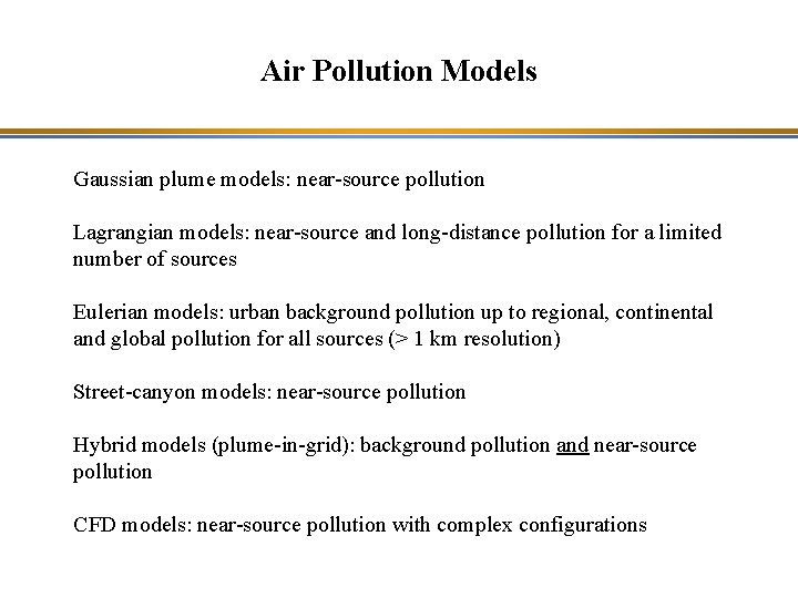
Air Pollution Models Gaussian plume models: near-source pollution Lagrangian models: near-source and long-distance pollution for a limited number of sources Eulerian models: urban background pollution up to regional, continental and global pollution for all sources (> 1 km resolution) Street-canyon models: near-source pollution Hybrid models (plume-in-grid): background pollution and near-source pollution CFD models: near-source pollution with complex configurations

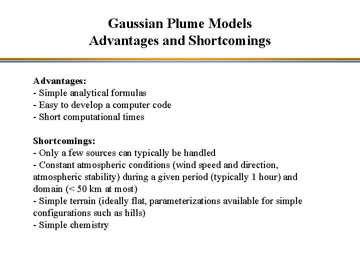
Gaussian Plume Models Advantages and Shortcomings Advantages: - Simple analytical formulas - Easy to develop a computer code - Short computational times Shortcomings: - Only a few sources can typically be handled - Constant atmospheric conditions (wind speed and direction, atmospheric stability) during a given period (typically 1 hour) and domain (< 50 km at most) - Simple terrain (ideally flat, parameterizations available for simple configurations such as hills) - Simple chemistry

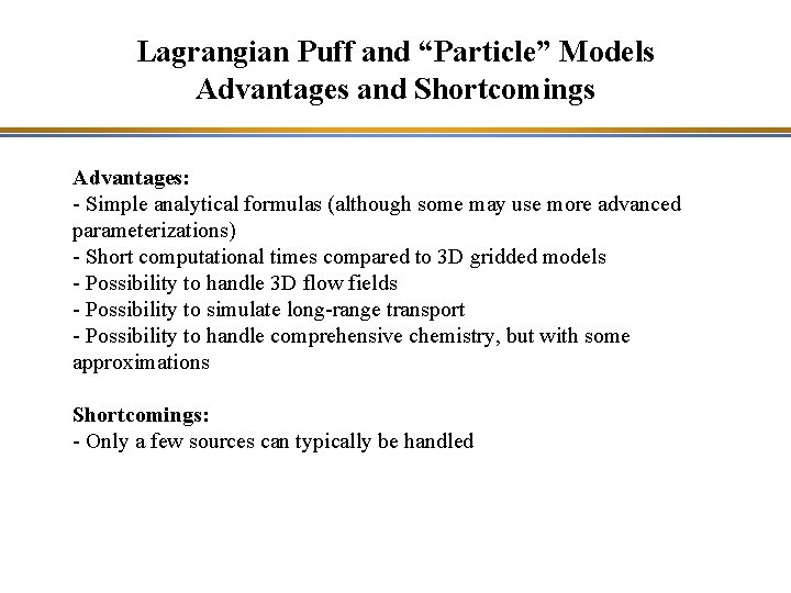
Lagrangian Puff and “Particle” Models Advantages and Shortcomings Advantages: - Simple analytical formulas (although some may use more advanced parameterizations) - Short computational times compared to 3 D gridded models - Possibility to handle 3 D flow fields - Possibility to simulate long-range transport - Possibility to handle comprehensive chemistry, but with some approximations Shortcomings: - Only a few sources can typically be handled

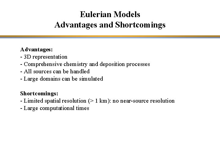
Eulerian Models Advantages and Shortcomings Advantages: - 3 D representation - Comprehensive chemistry and deposition processes - All sources can be handled - Large domains can be simulated Shortcomings: - Limited spatial resolution (> 1 km): no near-source resolution - Large computational times

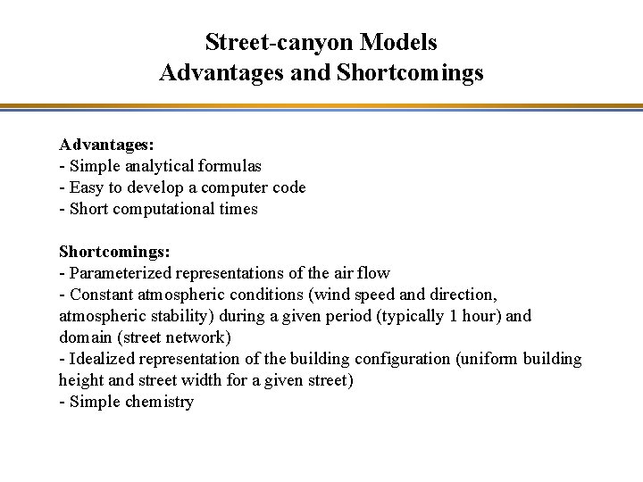
Street-canyon Models Advantages and Shortcomings Advantages: - Simple analytical formulas - Easy to develop a computer code - Short computational times Shortcomings: - Parameterized representations of the air flow - Constant atmospheric conditions (wind speed and direction, atmospheric stability) during a given period (typically 1 hour) and domain (street network) - Idealized representation of the building configuration (uniform building height and street width for a given street) - Simple chemistry

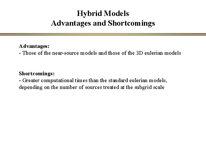
Hybrid Models Advantages and Shortcomings Advantages: - Those of the near-source models and those of the 3 D eulerian models Shortcomings: - Greater computational times than the standard eulerian models, depending on the number of sources treated at the subgrid scale

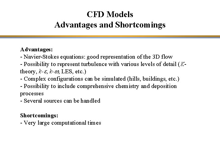
CFD Models Advantages and Shortcomings Advantages: - Navier-Stokes equations: good representation of the 3 D flow - Possibility to represent turbulence with various levels of detail (Ktheory, k-e, k-w, LES, etc. ) - Complex configurations can be simulated (hills, buildings, etc. ) - Possibility to include comprehensive chemistry and deposition processes - Several sources can be handled Shortcomings: - Very large computational times