Computer Graphics Lecture 37 CURVES III Taqdees A

Computer Graphics Lecture 37

CURVES III Taqdees A. Siddiqi cs 602@vu. edu. pk

The Tangent Vector

• Another way to define a space curve does not use intermediate points. It uses the tangents at each end of a curve, instead

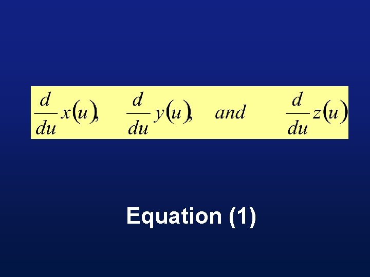
• Every point on a curve has a straight line associated with it called the tangent line, which is related to the first derivation of the Parametric functions x(u), y(u), and z(u)

Equation (1)

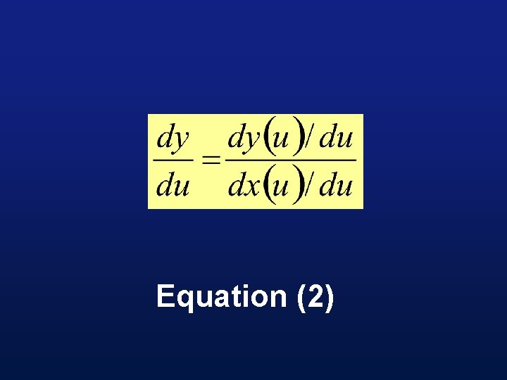
• From elementary calculus, we can compute, for example,

Equation (2)

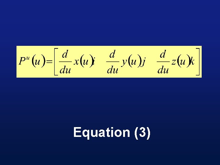
• We can treat as components of a vector along the tangent line to the curve. We call this the tangent vector, and define it as

Equation (3)

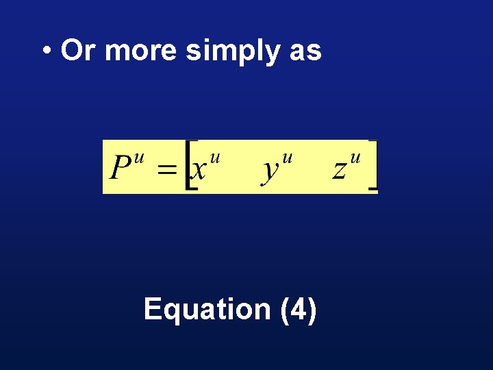
• Or more simply as Equation (4)

• (Here the superscript u indicates the first derivative operation with respect to the independent variable u). This is a very powerful idea, and we will now see how to use it to define a curve

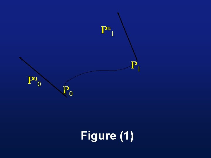
• We will still use the two end points, but instead of two intermediate points, we will use the tangent vectors at each end to supply the information we need to define a curve

• By manipulating these tangent vectors, we can control the slope at each end. The set of vectors , , , and are called the boundary conditions

• This method itself is called the cubic Hermite interpolation, after C. Hermite (1822 -1901) the French mathematician who made significant contributions to our understanding of cubic and quadratic polynomials.

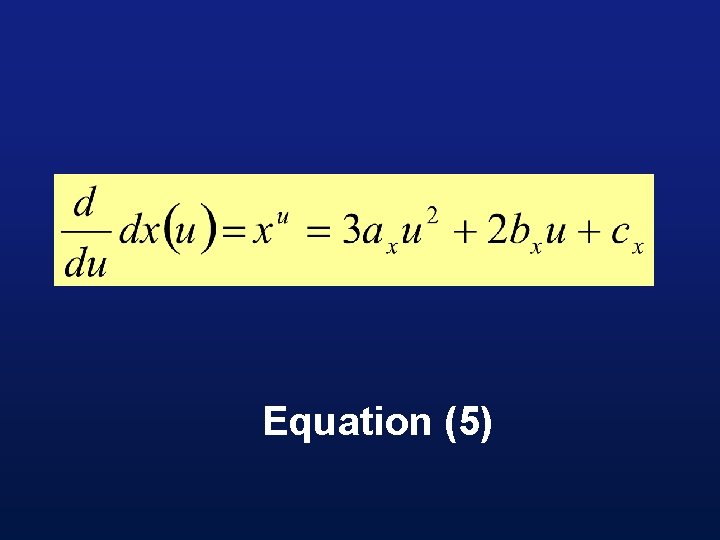
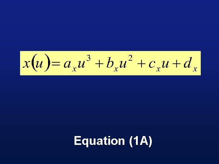
• We differentiate to obtain the x component of the tangent vector:

Equation (5)

Pu 1 Pu 0 P 0 Figure (1)

Equation (1 A)

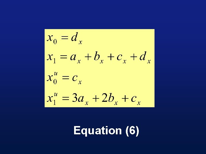
• Evaluating (1 A) and Equation 5 at u = 0, u = 1, yields

Equation (6)

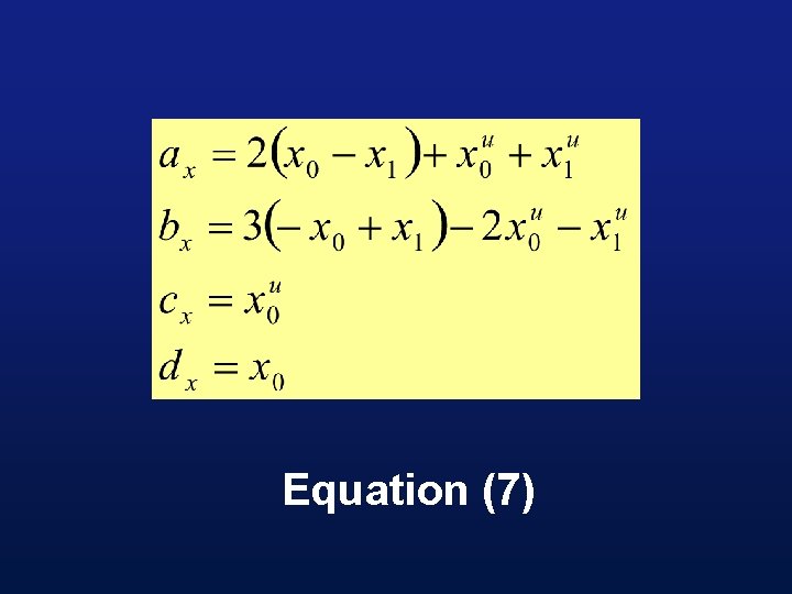
• Using these four equations in four unknowns, we solve for ax , bx , cx and dx in terms of the boundary conditions

Equation (7)

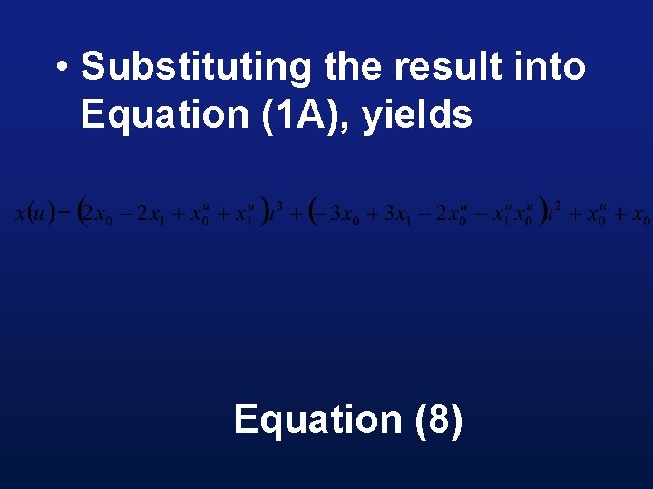
• Substituting the result into Equation (1 A), yields Equation (8)

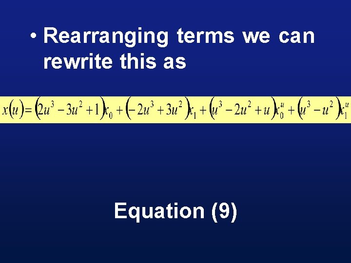
• Rearranging terms we can rewrite this as Equation (9)

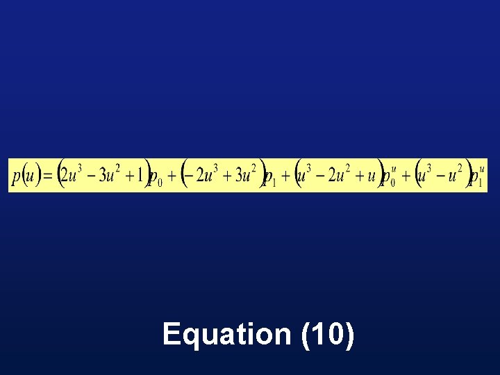
• Because y(u) and z(u) have equivalent forms, we can include them by rewriting Equation 9 in vector form:

Equation (10)

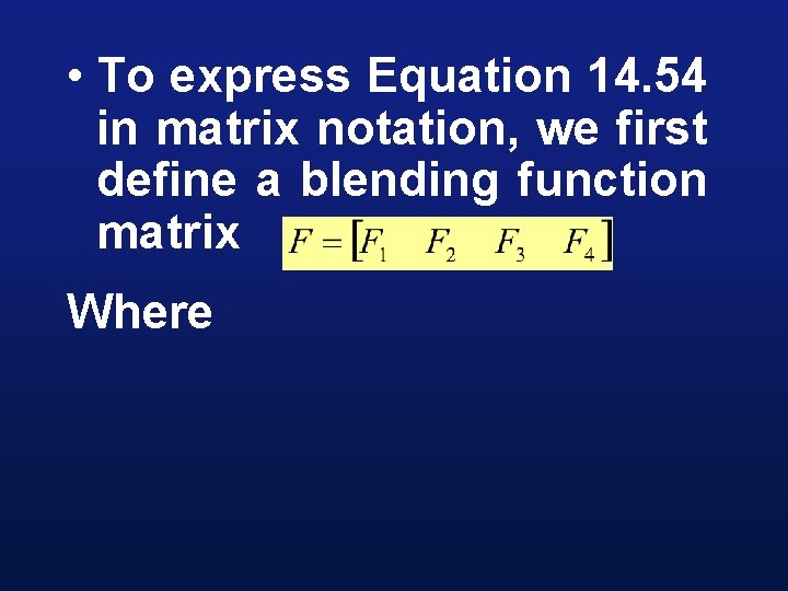
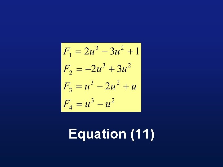
• To express Equation 14. 54 in matrix notation, we first define a blending function matrix Where

Equation (11)

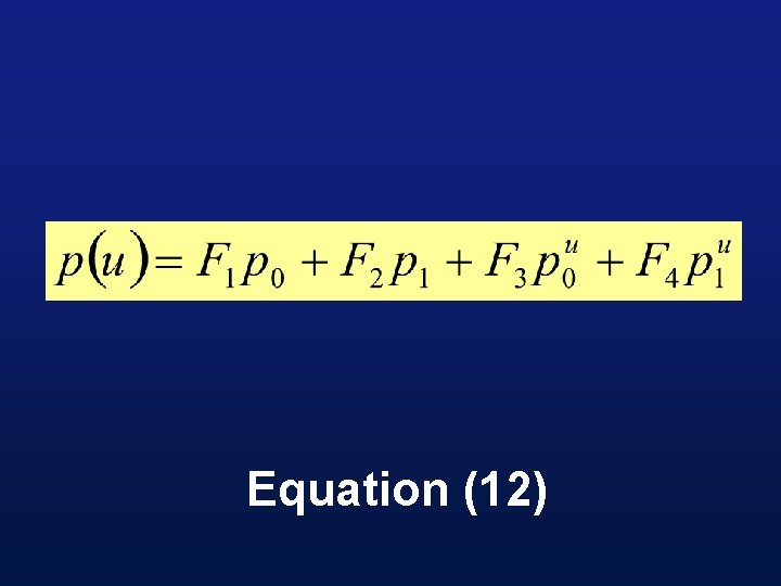
• These matrix elements are the polynomial coefficients of the vectors which we rewrite as:

Equation (12)

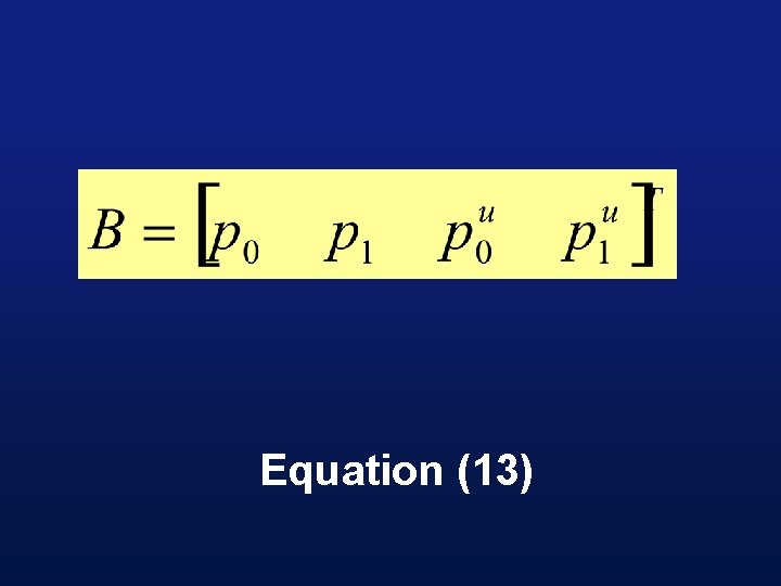
• If we assemble the vectors representing the boundary conditions into a matrix B,

Equation (13)

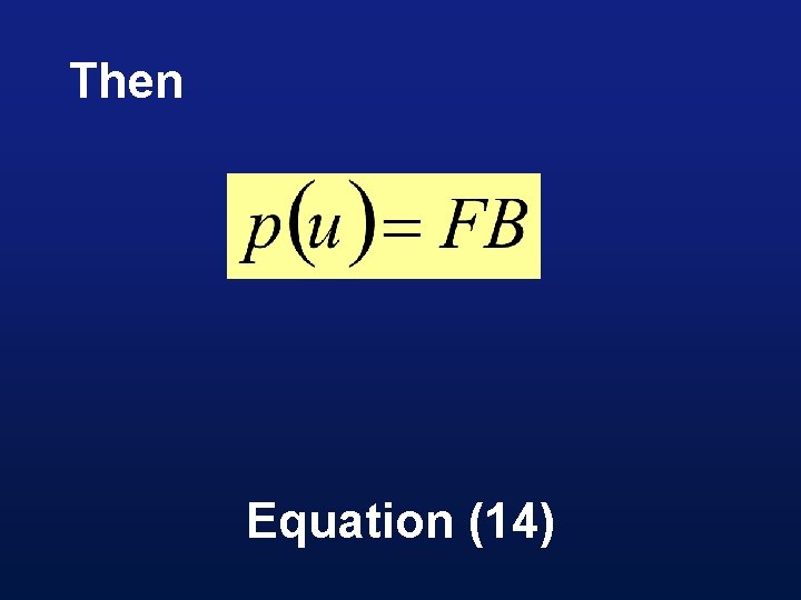
Then Equation (14)

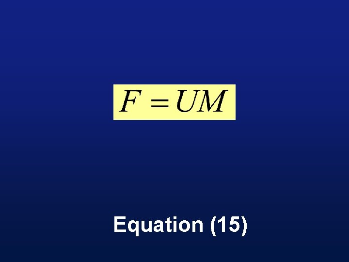
• Here again we write the matrix F as the product of two matrices, U and M, so that

Equation (15)

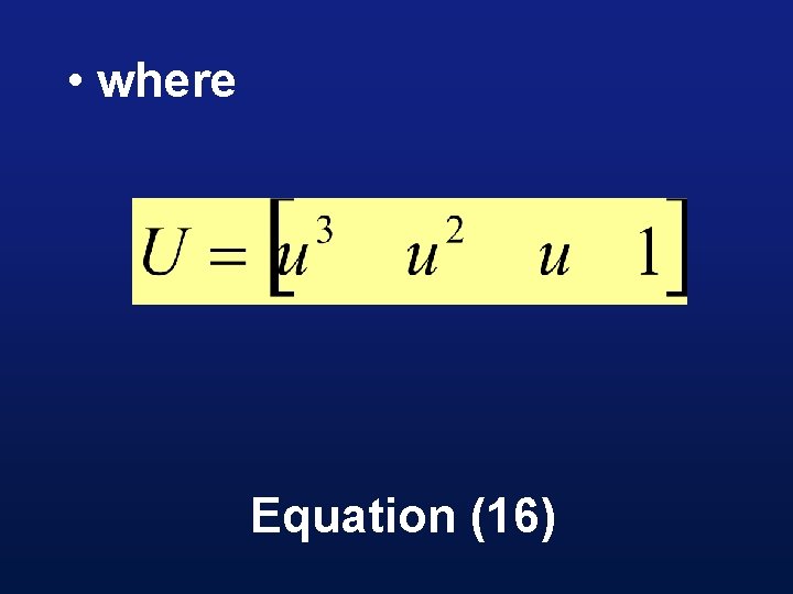
• where Equation (16)

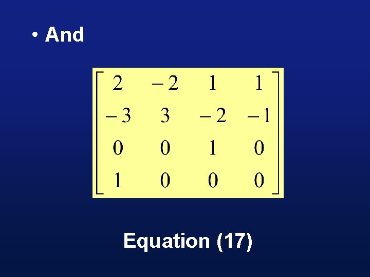
• And Equation (17)

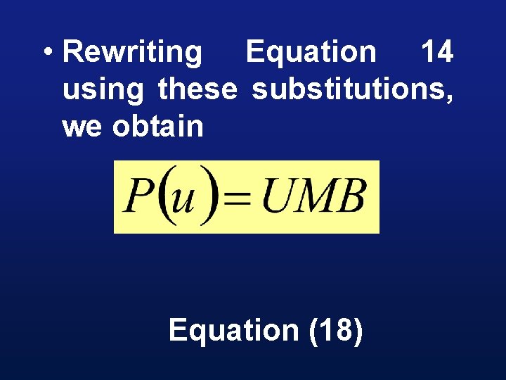
• Rewriting Equation 14 using these substitutions, we obtain Equation (18)

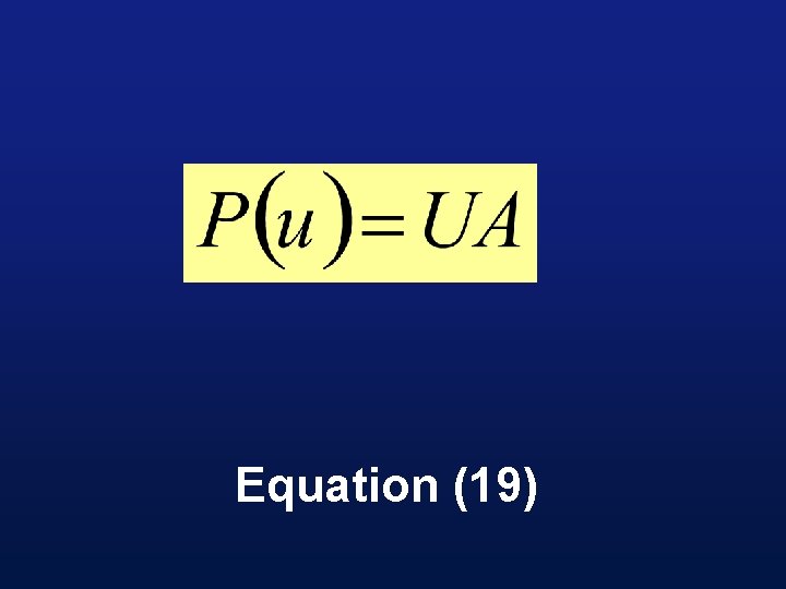
• It is easy to show the relationship between the algebraic and geometric coefficients for a space curve. Since

Equation (19)

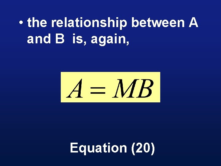
• the relationship between A and B is, again, Equation (20)

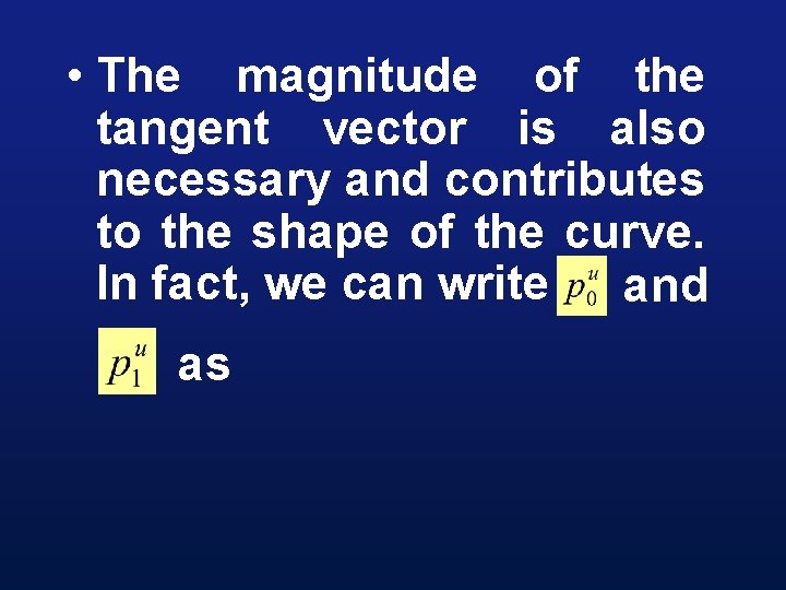
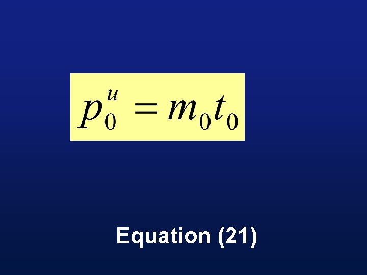
• The magnitude of the tangent vector is also necessary and contributes to the shape of the curve. In fact, we can write and as

Equation (21)

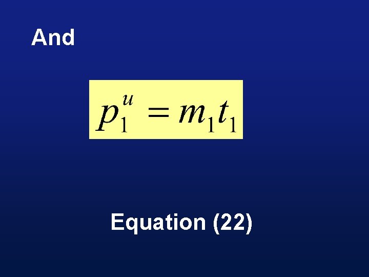
And Equation (22)

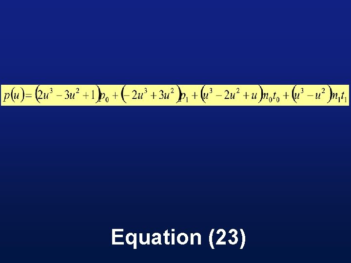
• Clearly, m 0, and m 1 are the magnitudes of and. • Using these relationships, we modify Equation 10 as follows:

Equation (23)

Computer Graphics Lecture 37

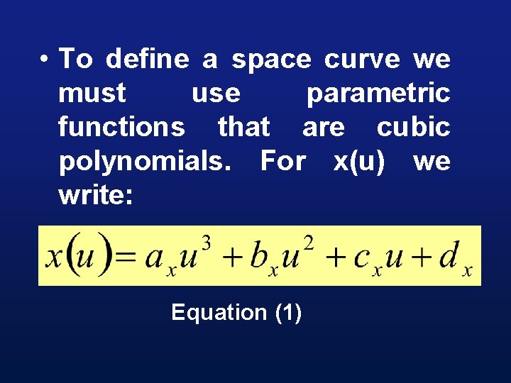
• To define a space curve we must use parametric functions that are cubic polynomials. For x(u) we write: Equation (1)

• A space curve is not confined to a plane. It is free to twist through space.

Space Curves

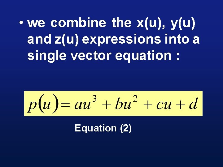
• we combine the x(u), y(u) and z(u) expressions into a single vector equation : Equation (2)

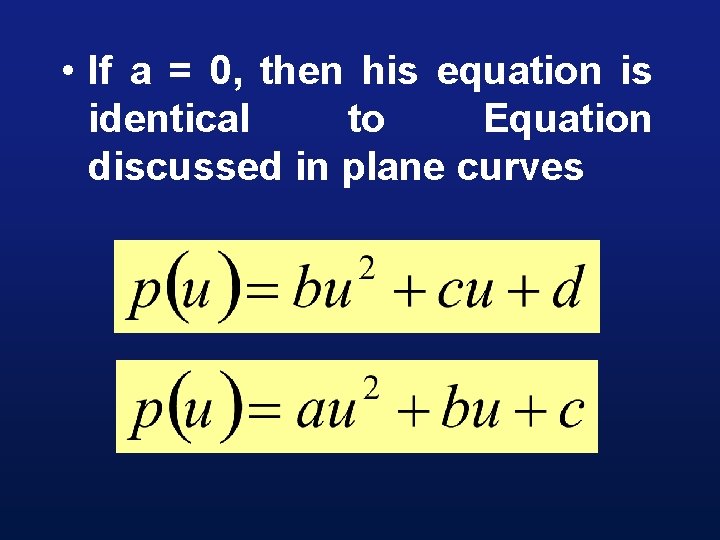
• If a = 0, then his equation is identical to Equation discussed in plane curves

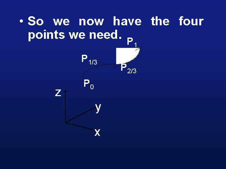
• So we now have the four points we need. P 1/3 z P 0 y x P 2/3

• So we now have the four points we need. P 1/3 z P 0 y x P 2/3

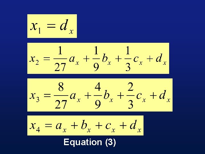
Equation (3)

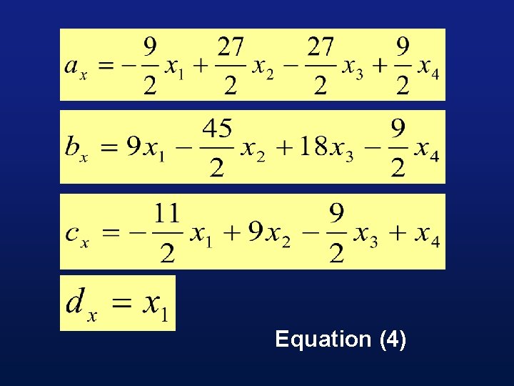
Equation (4)

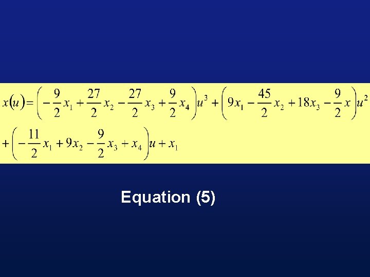
Equation (5)

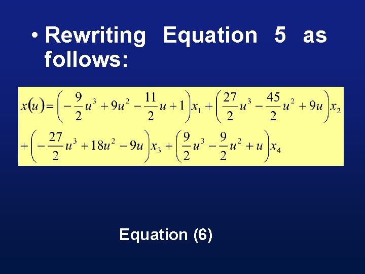
• Rewriting Equation 5 as follows: Equation (6)

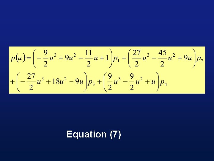
Equation (7)

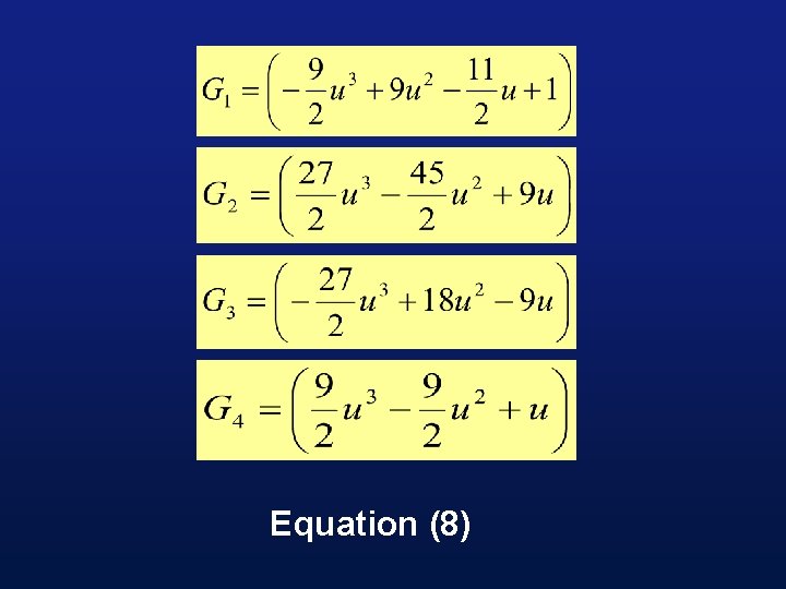
• This means that, given four point assigned successive values of u (in this case at u=0, 1/3, 2/3 & 1), equation 7 produces a curve that starts at p 1, passes through p 2 and p 3, and ends at p 4.

• Now let’s take one more step towards a more compact notation. Using the four parametric functions appearing in Equation 7, we define a new matrix, where

Equation (8)

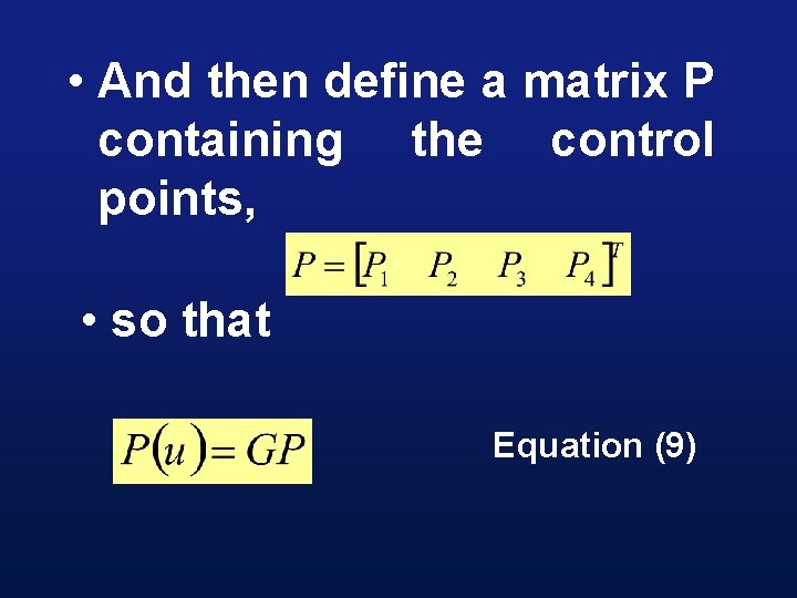
• And then define a matrix P containing the control points, • so that Equation (9)

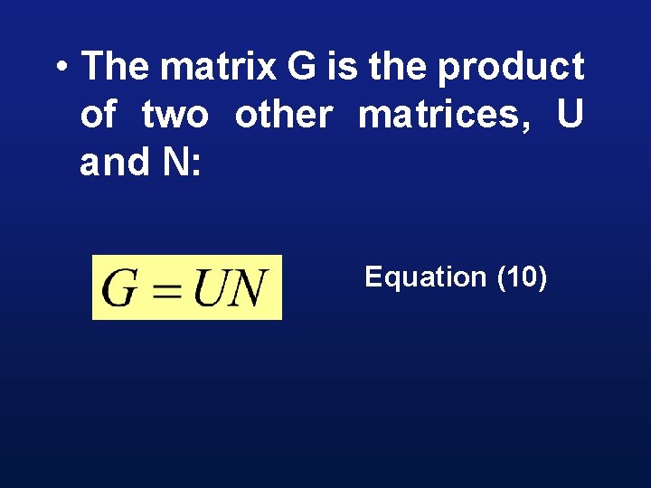
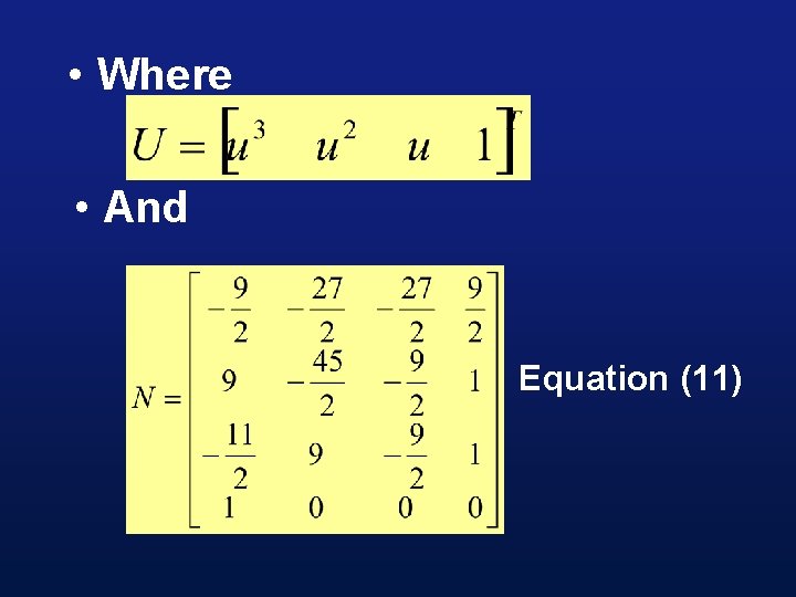
• The matrix G is the product of two other matrices, U and N: Equation (10)

• Where • And Equation (11)

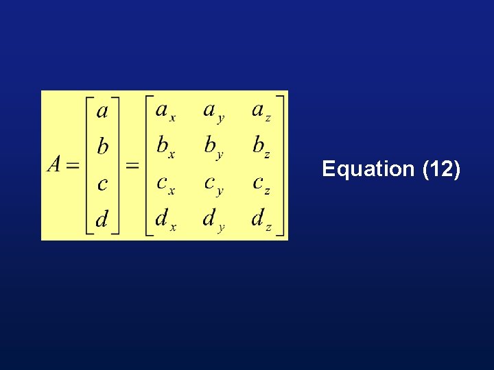
Equation (12)

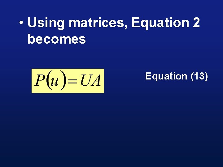
• Using matrices, Equation 2 becomes Equation (13)

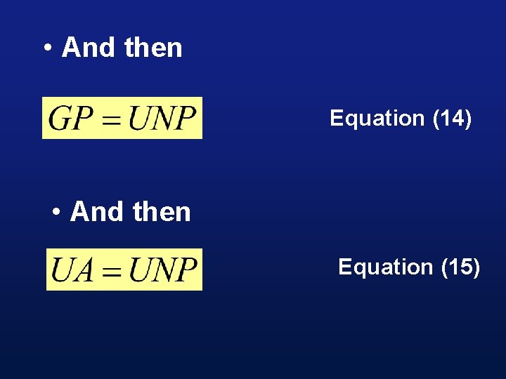
• And then Equation (14) • And then Equation (15)

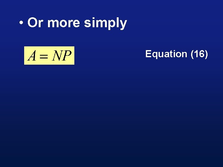
• Or more simply Equation (16)

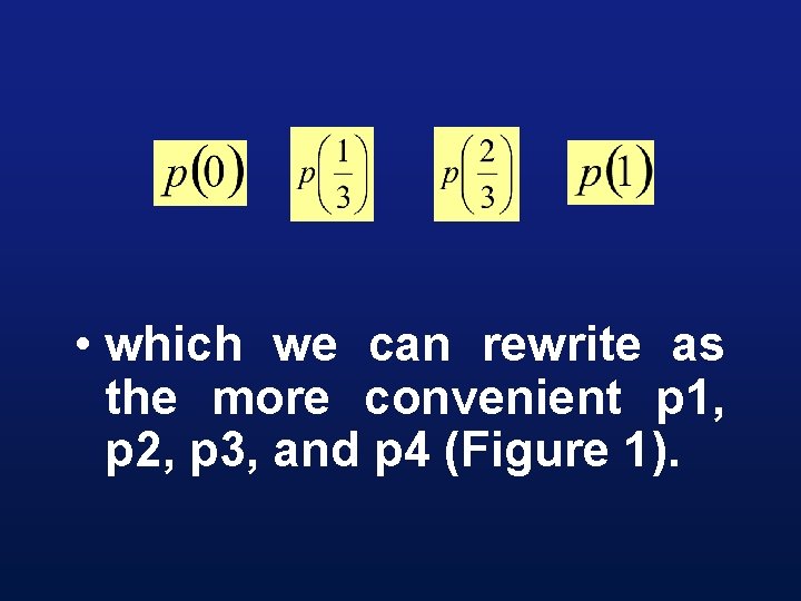
• which we can rewrite as the more convenient p 1, p 2, p 3, and p 4 (Figure 1).