Raster Scan Graphics DDA Line Drawing Algorithm 1

Raster Scan Graphics

DDA Line Drawing Algorithm 1. Read line end points(x 1, y 1) and (x 2, y 2) such that they are not equal. 2. dy=|y 2 -y 1| and dx=|x 2 -x 1| 3. if(abs(dx)>abs(dy)) length=abs(dx); else length=abs(dy); 4. Calculate xincrement and yincrement. xinc=dx/(float)length; yinc=dy/(float)length; 5. x=x 1 y=y 1 putpixel(x, y, 10); 6. Continue process till I reaches to length as for(i=0; i<length; i++) { putpixel(x, y, 10); x=x+xinc; y=y+yinc; delay(10); }

DDA Line Drawing Program #include<stdio. h> #include<conio. h> #include<graphics. h> void main() { int x 1, y 1, x 2, y 2, dx, dy, length, i; float x, y, xinc, yinc; int gd=DETECT, gm; initgraph(&gd, &gm, "c: \turboc 3\bgi"); printf("Enter the starting coordinates"); scanf("%d%d", &x 1, &y 1); printf("Enter the ending coordinates"); scanf("%d%d", &x 2, &y 2); dx=x 2 -x 1; dy=y 2 -y 1; if(abs(dx)>abs(dy)) length=abs(dx); else length=abs(dy); xinc=dx/(float)length; yinc=dy/(float)length; x=x 1; y=y 1; putpixel(x, y, 10); for(i=0; i<length; i++) { x=x+xinc; y=y+yinc; putpixel(x, y, 10); delay(10); } getch(); closegraph(); }

Advantages and Disadvantages • Advantages 1. It is the simplest algorithm and it does not require special skills for implementation. 2. It is a faster method for calculating pixel positions. • Disadvantages 1. Floating point arithmetic in DDA algorithm is still timeconsuming. 2. The algorithm is orientation dependent. Hence end point accuracy is poor.

Bresenham’s Line Drawing Algorithm 1. Read line end points(x 1, y 1) and (x 2, y 2) such that they are not equal. 2. dy=|y 2 -y 1| and dx=|x 2 x 1| 3. e=2*(dy-dx); x=x 1; y=y 1; 4. while(x<=x 2) perform following { if(e<0) { x=x+1; 5. y=y; e=e+2*dy; } 6. else { x=x+1; y=y+1; e=e+2*(dy-dx); } putpixel(x, y, 15); } 7. Stop.

Bresenham’s Line Drawing Program #include<stdio. h> #include<conio. h> #include<graphics. h> #include<math. h> void main() { int length, dx, dy, x 1, y 1, x 2, y 2, e; float x, y; int gd=DETECT, gm; initgraph(&gd, &gm, "c: //Turboc 3//BGI"); printf("n enter coordinates of x 1, y 1, x 2, y 2"); scanf("%d%d", &x 1, &y 1, &x 2, &y 2); dx=x 2 -x 1; dy=y 2 -y 1; e=2*(dy-dx); x=x 1; y=y 1; while(x<=x 2) { if(e<0) { x=x+1; y=y; e=e+2*dy; } else { x=x+1; y=y+1; e=e+2*(dy-dx); } putpixel(x, y, 15); } getch(); closegraph(); }

DDA Line Drawing Algorithm Bresenhams Line Drawing Algorithm Arithmetic uses floating points Integer points Operations Uses multiplication and division in its operations. Uses only subtraction and addition in its operations. Speed slower than Bresenham’s algorithm faster than DDA Accuracy & Efficiency Drawing Round Off Expensive not as accurate and efficient more efficient &much accurate DDA algorithm can draw Draw circles and curves with circles and curves but that are much more accuracy than DDA not as accurate as Bresenham’s algorithm. Bresenhams’ algorithm does not DDA algorithm round off the round off but takes the coordinates to integer that incremental value in its is nearest to the line. operation. Expensive Less Expensive

Symmetry of circle • A circle is a geometric figure which is round, and can be divided into 360 degrees. A circle is a symmetrical figure which follows 8 -way symmetry. • 8 -Way symmetry: Any circle follows 8 -way symmetry. This means that for every point (x, y) 8 points can be plotted. These (x, y), (y, x), (-x, y), (-x, -y), (-y, -x), (x, -y). Drawing a circle: To draw a circle we need two things, the coordinates of the Centre and the radius of the circle. Here r is the radius of the circle. If the circle has origin (0, 0) as its Centre then the above equation can be reduced to x 2+ y 2=r 2

Bresenham’s Circle Drawing Algorithm 1. Read the radius of circle. 2. Calculate initial decision parameter di=3 -2 r 3. x=0 and y=r [initialize the starting point] 4. while(x<y) { Plot(x, y)//plot point(x, y) and other 7 points in all octant x=x+1; if(d<0) { d=d+(4*x)+6; } else { y=y-1; d=d+4*(x-y)+10; } Plot(x, y) }// end of while 5. Stop.

Bresenham’s Circle Drawing Program #include<stdio. h> #include<conio. h> #include<math. h> #include<dos. h> #include<graphics. h> void bressn(int, int); void plot(int, int); void plot(int xc, int yc, int x, int y) { putpixel(xc+x, yc+y, WHITE); putpixel(xc-x, yc+y, RED); putpixel(xc-x, yc-y, GREEN); putpixel(xc+x, yc-y, YELLOW); putpixel(xc+y, yc+x, WHITE); putpixel(xc-y, yc+x, GREEN); putpixel(xc-y, yc-x, YELLOW); putpixel(xc+y, yc-x, RED); } void bressn(int xc, int yc, int r) { int d, x, y; d=3 -(2*r); x=0; y=r; while(x<y) { if(d<0) { d=d+(4*x)+6; } else { d=d+4*(x-y)+10; y=y-1; } x=x+1; plot(xc, yc, x, y); } }

void main() { int gd, gm; int xc, yc, radius; detectgraph(&gd, &gm); initgraph(&gd, &gm, "c: \turboc 3\bgi"); printf("n enter xc, yc, radius"); scanf("%d%d%d", &xc, &yc, &radius); bressn(xc, yc, radius); getch(); closegraph(); }

Midpoint Circle Drawing Algorithm 1. Read the radius of circle. 2. x=0 and y=r [initialize the starting point] p=1 -r; plot (x, y) )//plot point(x, y) and other 7 points in all octant. 3. while(x<y) { if(p<0) { x++; p=p+2*x+1; } else { x++; y--; p=p+2*(x-y)+1; } plot (x, y) )//plot point(x, y) and other 7 points in all octant. } 4. Stop

Midpoint Circle Drawing Program #include<graphics. h> #include<stdio. h> #include<conio. h> #include<math. h> void plot(int xc, int yc, int x, int y); int main() { int gd, gm, xc, yc, r, x, y, p; detectgraph(&gd, &gm); initgraph(&gd, &gm, "C: //Turbo. C 3//BGI"); printf("Enter center of circle : "); scanf("%d%d", &xc, &yc); printf("Enter radius of circle : "); scanf("%d", &r); x =0; y=r; p=1 -r; plot(xc, yc, x, y); while(x<y) { if(p<0) { x++; p=p+2*x+1; } else { x++; y--; p=p+2*(x-y)+1; } plot(xc, yc, x, y); }

getch(); closegraph(); return 0; } void plot(int xc, int yc, int x, int y) { putpixel(xc+x, yc+y, WHITE); putpixel(xc+x, yc-y, WHITE); putpixel(xc-x, yc+y, WHITE); putpixel(xc-x, yc-y, WHITE); putpixel(xc+y, yc+x, WHITE); putpixel(xc+y, yc-x, WHITE); putpixel(xc-y, yc+x, WHITE); putpixel(xc-y, yc-x, WHITE); }

Types of Polygon • Convex Polygon • Concave Polygon The difference between convex and concave polygons lies in the measures of their angles. For a polygon to be convex, all of its interior angles must be less than 180 degrees. Otherwise, the polygon is concave.

Polygon Inside-Outside Test This method is also known as counting number method. While filling an object, we often need to identify whether particular point is inside the object or outside it. There are two methods by which we can identify whether particular point is inside an object or outside. • Odd-Even Rule • Nonzero winding number rule

Odd-Even Rule In this technique, we will count the edge crossing along the line from any point (x, y) to infinity. If the number of interactions is odd, then the point (x, y) is an interior point; and if the number of interactions is even, then the point (x, y) is an exterior point. The following example depicts this concept. From the above figure, we can see that from the point (x, y), the number of interactions point on the left side is 5 and on the right side is 3. From both ends, the number of interaction points is odd, so the point is considered within the object.

Nonzero Winding Number Rule This method is also used with the simple polygons to test the given point is interior or not. • Give the value 1 to all the edges which are going to upward direction and all other -1 as direction values. • Check the edge direction values from which the scan line is • passing and sum up them. • If the total sum of this direction value is non-zero, then this point to be tested is an interior point, otherwise it is an exterior point. In the above figure, we sum up the direction values from which the scan line is passing then the total is 1 – 1 + 1 = 1; which is non-zero. So the point is said to be an interior point.

Polygon Filling • One way to fill polygon is to start from given “seed”, point known to be inside the polygon and highlight outward from this point i. e. neighboring pixels until we encounter the boundary pixels. This approach is called seed fill. • Seed fill algorithm further classified as flood fill and boundary fill algorithm. • Algorithms the fill interior defined regions are flood fill algorithms; those that fill boundary defined regions are called boundary fill algorithm. Another approach to fill the polygon is to apply the inside test i. e. to check whether the pixel is inside the polygon or outside the polygon and then highlight pixels which lie inside the polygon. This approach is known as scan-line algorithm.

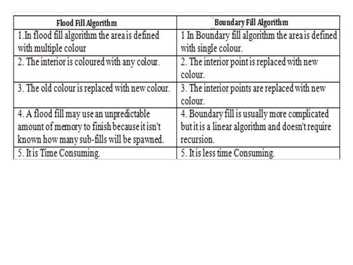
Flood Fill Flood fill colors an entire area in an enclosed figure using a single color. The algorithm works in a manner so as to give color to all the pixels inside the boundary the same color leaving the boundary and the pixels outside. • Flood fill algorithm is used for filling the interior of a polygon. • Used when an area defined with multiple color boundaries. • Start at a point inside a region− Replace a specified interior color (old color) with fill color • Fill the 4−connected or 8−connected region until all interior points being replaced.

4−Connected Regions From a given pixel, the region that you can get to by a series of 4 way moves (north, south, east, west) void fillcolor(int x, int y, int old_color, int new_color) { if(getpixel(x, y)==old_color) { delay(5); putpixel(x, y, new_color); fillcolor(x+1, y, old_color, new_color); fillcolor(x-1, y, old_color, new_color); fillcolor(x, y+1, old_color, new_color); fillcolor(x, y-1, old_color, new_color); } }

#include<stdio. h> #include<conio. h> #include<graphics. h> #include<dos. h> void fillcolor(int, int); void main() { int gd, gm; detectgraph(&gd, &gm); initgraph(&gd, &gm, "c: \turboc 3\bgi"); rectangle(50, 100, 100); fillcolor(55, 0, 11); getch(); closegraph(); } void fillcolor(int x, int y, int old_color, int new_color) { if(getpixel(x, y)==old_color) { delay(5); putpixel(x, y, new_color); fillcolor(x+1, y, old_color, new_color) ; fillcolor(x-1, y, old_color, new_color); fillcolor(x, y+1, old_color, new_color); fillcolor(x, y-1, old_color, new_color); } }

8−Connected Regions From a given pixel, the region that you can get to by a series of 8 -way moves (north, south, east, west, NE, NW, SE, SW) void fillcolor(int x, int y, int old_color, int new_color) { if(getpixel(x, y)==old_color) { delay(5); putpixel(x, y, new_color); fillcolor(x+1, y, old_color, new_color); fillcolor(x-1, y, old_color, new_color); fillcolor(x, y+1, old_color, new_color); fillcolor(x, y-1, old_color, new_color); fillcolor(x+1, y+1, old_color, new_color); fillcolor(x+1, y-1, old_color, new_color); fillcolor(x-1, y+1, old_color, new_color); } }

#include<stdio. h> #include<conio. h> #include<graphics. h> #include<dos. h> void fillcolor(int, int); void main() { int gd, gm; detectgraph(&gd, &gm); initgraph(&gd, &gm, "c: \turboc 3\bgi"); rectangle(50, 100, 100); fillcolor(55, 0, 11); getch(); closegraph(); } void fillcolor(int x, int y, int old_color, int new_color) { if(getpixel(x, y)==old_color) { delay(5); putpixel(x, y, new_color); fillcolor(x+1, y, old_color, new_color); fillcolor(x-1, y, old_color, new_color); fillcolor(x, y+1, old_color, new_color); fillcolor(x, y-1, old_color, new_color); fillcolor(x+1, y+1, old_color, new_color); fillcolor(x+1, y-1, old_color, new_color); fillcolor(x-1, y+1, old_color, new_color); } }

Boundary Fill Start at a point inside the figure and paint with a particular color. Filling continues until a boundary color is encountered. • In boundary fill algorithm Recursive method is used to fill the whole boundary. • Start at a point inside a region. • Paint the interior outward toward the boundary. • The boundary is specified in a single color.

4 -connected boundary fill Algorithm: boundary_fill(x, y, f_colour, b_colour) { if(getpixel(x, y)! = b_colour && getpixel(x, y)! = f_colour) { putpixel(x, y, f_colour); boundary_fill(x + 1, y, f_colour, b_colour); boundary_fill(x, y + 1, f_colour, b_colour); boundary_fill(x -1, y, f_colour, b_colour); boundary_fill(x, y – 1, f_colour, b_colour); } }

#include<stdio. h> #include<conio. h> #include<graphics. h> #include<dos. h> void boundary_fill (int, int); void main() { int gd, gm; detectgraph(&gd, &gm); initgraph(&gd, &gm, "c: \turboc 3 \bgi"); rectangle(50, 100, 100); boundary_fill(55, 6, 15); getch(); closegraph(); } void boundary_fill(int x, int y, int fcolor, int bcolor) { if((getpixel(x, y)!=bcolor) && (getpixel(x, y)!=fcolor)) { delay(5); putpixel(x, y, fcolor); boundary_fill(x+1, y, fcolor, bcolor); boundary_fill(x-1, y, fcolor, bcolor); boundary_fill(x, y+1, fcolor, bcolor); boundary_fill(x, y-1, fcolor, bcolor); } }

8 -connected boundary fill Algorithm: boundary_fill(x, y, f_colour, b_colour) { if(getpixel(x, y)! = b_colour && getpixel(x, y)! = f_colour) { putpixel(x, y, f_colour); boundary_fill(x + 1, y, f_colour, b_colour); boundary_fill(x - 1, y, f_colour, b_colour); boundary_fill(x, y + 1, f_colour, b_colour); boundary_fill(x, y - 1, f_colour, b_colour); boundary_fill(x + 1, y + 1, f_colour, b_colour); boundary_fill (x - 1, y - 1, f_colour, b_colour); boundary_fill(x + 1, y - 1, f_colour, b_colour); boundary_fill(x - 1, y + 1, f_colour, b_colour); } }

#include<stdio. h> #include<conio. h> #include<graphics. h> #include<dos. h> void boundary_fill(int, int); void main() { int gd, gm; detectgraph(&gd, &gm); initgraph(&gd, &gm, "c: \turboc 3 bgi"); rectangle(50, 100, 100); boundary_fill(55, 6, 15); getch(); closegraph(); } void boundary_fill(int x, int y, int fcolor, int bcolor) { if((getpixel(x, y)!=bcolor)&&(getpixel (x, y)!=fcolor)) { delay(5); putpixel(x, y, fcolor); boundary_fill(x+1, y, fcolor, bcolor); boundary_fill(x-1, y, fcolor, bcolor); boundary_fill(x, y+1, fcolor, bcolor); boundary_fill(x, y-1, fcolor, bcolor); boundary_fill(x+1, y+1, fcolor, bcolor); boundary_fill(x-1, y+1, fcolor, bcolor); boundary_fill(x+1, y-1, fcolor, bcolor); boundary_fill(x-1, y-1, fcolor, bcolor); } }

Scan Conversion • The process of representing continuous graphics objects as a collection of discrete pixels is called scan conversion. Scan conversion serves as a bridge between TV and computer graphics technology. • Scan conversion or scan converting rate is a video processing technique for changing the vertical / horizontal scan frequency of video signal for different purposes and applications. • The device which performs this conversion is called a scan converter. • The application of scan conversion: video projectors, cinema equipment, TV and video capture cards, standard and HDTV televisions, LCD monitors, radar displays and many different aspects of picture processing.

There are two distinct methods for changing a picture's data rate: Analog Methods (Non retentive, memory-less or real time method) • This conversion is done using large numbers of delay cells and is appropriate for analog video. It may also be performed using a specialized scan converter vacuum tube. • In this case polar coordinates (angle and distance) data from a source such as a radar receiver, so that it can be displayed on a raster scan (TV type) display. Digital methods (Retentive or buffered method) • In this method, a picture is stored in a line or frame buffer with n 1 speed (data rate) and is read with n 2 speed.

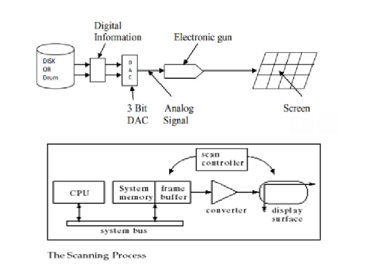
Frame Buffer • Each screen pixel corresponds to a particular entry in a 2 D array residing in memory. This memory is called a frame buffer or a bit map. • The number of rows in the frame buffer equals to the number of raster lines on the display screen. The number of columns in this array equals to the number of pixels on each raster line. • Frame buffer is a large part of computer memory used to store display image. Different kind of memory can be used for frame buffers like drums, disk or IC – shift registers. • To generate a pixel of desired intensity to read the disk or drum. The information stored in disk or drum is in digital for, hence it is necessary to convert it into analog from using DAC and then this analog signal is used to generate the pixel.

Character Generation Most of the times characters are built into the graphics display devices, usually as hardware but sometimes through software. There are basic three methods: • • • Stroke method Starburst method Bitmap method

Stroke Method This method uses small line segments to generate a character. • The small series of line segments are drawn like a strokes of a pen to form a character as shown in figure. • We can build our own stroke method. • By calling a line drawing algorithm. • Here it is necessary to decide which line segments are needed for each character and • Then drawing these segments using line drawing algorithm. • This method supports scaling of the character. • It does this by changing the length of the line segments used for character drawing.

Starburst method

In this method a fix pattern of line segments are used to generate characters. • As shown in figure, there are 24 line segments. • Out of 24 line segments, segments required to display for particular character, are highlighted • This method is called starburst method because of its characteristic appearance. This method of character generation has some disadvantages. They are 1. The 24 -bits are required to represent a character. Hence more memory is required 2. Requires code conversion software to display character from its 24 -bit code 3. Character quality is poor. It is worst for curve shaped characters.

Bitmap Method Also known as dot matrix because in this method characters are represented by an array of dots in the matrix form. • It’s a two dimensional array having columns and rows : 5 X 7 as shown in figure. • 7 X 9 and 9 X 13 arrays are also used. • Higher resolution devices may use character array 100 X 100.