Computer Graphics Lecture 35 CURVES Taqdees A Siddiqi

Computer Graphics Lecture 35

CURVES Taqdees A. Siddiqi cs 602@vu. edu. pk

Curves

We all know what a curve is. Today we will explore the mathematical definition of a curve in a form that is very useful to geometric modeling and other computer graphics applications

The mathematics of parametric equations is the basis for Bezier, NURBS (Non Uniform Rational Beta Splines), and Hermite curves

Parametric Equations of a Curve

A parametric curve is one whose defining equations are given in terms of a single, common, independent variable called the parametric variable.

We have already encountered parametric variables in earlier discussions of vectors, lines, and planes.

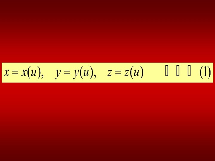
In three-dimensional space each point on curve has unique set of coordinates: each coordinate is controlled by a separate parametric equation, whose general form looks like

where x(u) stands for some as yet unspecified function in which u is the independent variable;

for example, x(u) = au 2 + bu + c, and similarly for y(u) and z(u). It is important to understand that each of these is an independent expression

The dependent variables are the x, y, and z coordinates themselves, because their values depend on the value of the parametric variable u

Figure 1: point of a curve defined by a vector.

Each point on a curve is defined by a vector p (figure 1). The components of this vector are x(u), y(u), and z(u). we express this as

which says that the vector p is a function of the parametric variable u.

There is a lot of information in equation 2. when we expand it into component form, it becomes

There are only a few simple rules that we must follow to design these mathematical functions

1) define each component by a single, common parametric variable, and 2) make sure that each point on the curve corresponds to a unique value of the parametric variable.

Plane Curves

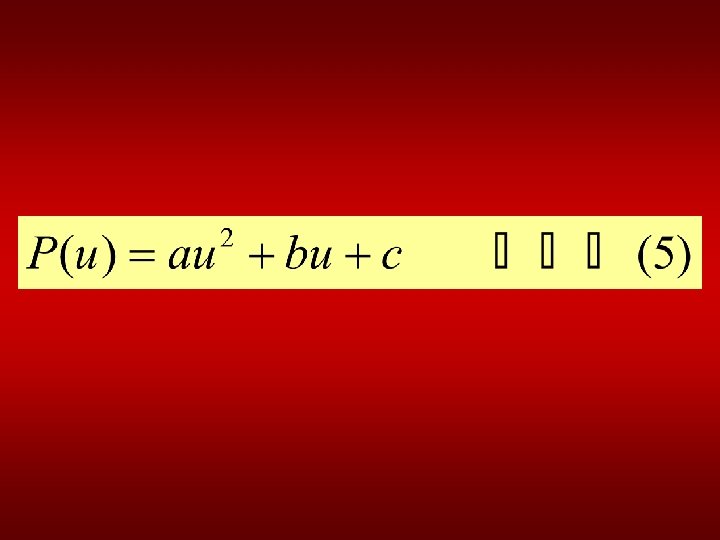
To define plane curves, we use parametric functions that are second-degree polynomials:

• where the a, b, and c terms are constant coefficients. • We can combine x(u), y(u), z(u), and their respective coefficients into an equivalent, more concise, vector equation:

We allow the parametric variable to take on values only in the interval 0 u 1.

It can generate conic curves but it cannot generate curve with an inflection point, like an S-shaped curve, no matter what values we select for the coefficients a, b, c. to do this requires a cubic polynomial.

To one of the end points we assign u = 0, and to the other u = 1. To the intermediate point, we arbitrarily assign u = 0. 5. We can write these points as

• P 0 = [x 0 y 0 • P 0. 5 = [x 0. 5 y 0. 5 • P 1 = [x 1 y 1 z 0] z 0. 5] …(6) z 1]

• Where the subscripts indicate the value of the parametric variable at each point. • Now we solve equations 4 for the ax, bx, …, cz coefficients in terms of these points. Thus, for x at u = 0, u =0. 5, and u =1, we have

• x 0 = cx • x 0. 5 = 0. 25 ax + 0. 5 bx + cx …(7) • x 1 = a x + b x + cx • with similar equations for y, and z.

Figure 2: A plane curve defined by three points

• Next we solve these three equations in three unknowns for ax, bx, and cx, finding • ax = 2 x 0 - 4 x 0. 5 + 2 x 1 • bx = -3 x 0 + 4 x 0. 5 + x 1 …(8) • cx = x 0

• Substituting this result in to equation 4 yields • x(u) = (2 x 0 - 4 x 0. 5 + 2 x 1 ) u 2 + (-3 x 0 + 4 x 0. 5 - x 1) u + x 0 …(9)

• Again, there are equivalent expressions for y(u) and z(u). • We rewrite equation 9 as follows:

x(u) = (2 u 2 – 3 u + 1) x 0 + (-4 u 2 + 4 u)x 0. 5 + 2 (2 u – u) x 1 …(10)

• Using this result and equivalent expressions for y(u) and z(u), we combine them into a single vector equation:

P(u) = (2 u 2 – 3 u + 1) P 0 + (-4 u 2 + 4 u)P 0. 5 + 2 (2 u – u) P 1 …(11)

Equation 11 produces the same curve as Equation 5. The curve will always lie in a plane no matter what three points we choose.

Furthermore, it is interesting to note that the point P 0. 5 which is on the curve at u= 0. 5, is not necessarily half way along the length of the curve between p 0 and p 1

Figure 3: Curve defined by three non-uniformly spaced points.

Equation 5 is the algebraic form and equation 11 is the geometric form. Each of these equations can be written more compactly with matrices

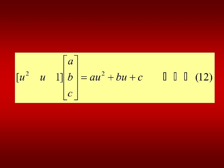
So now we rewrite equation 5 using the following substitutions:

And finally we obtain

Remember that A is actually a matrix of vectors, so that

• The nine terms on the right are called the algebraic coefficients. • Next, we convert equation 11 into matrix form. The right-hand side looks like the product of two matrices

and This means that

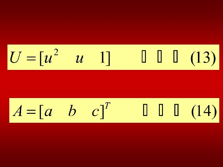
Using the following substitutions

and

where P is the control point matrix and the nine terms on the right are its elements or the geometric coefficients, we can now write

• This is the matrix version of the geometric form. • Because it is the same curve in algebraic form, p(u)=UA, or geometric form, p(u)=FP, we can write

The F matrix is itself the product of two other matrices

The matrix on the left we recognize as U, and we can denote the other matrix as

This means that

Using this we substitute appropriately to find

Pre-multiplying each side of this equation by 1/U yields

This expresses a simple relationship between the algebraic and geometric coefficients

Or

The matrix M is called a basis transformation matrix, and F is called a blending function matrix.

Computer Graphics Lecture 35